SDSC6007 Course 1

#sdsc6007

Introduction

The Discrete-Time Dynamic System

The system has the form

$$x_{k + 1} = f_{k} (x_k, u_k, w_k ), k = 0, 1, . . . , N − 1,$$

where

• $k$ : index of discrete time

• $N$ : the horizon or number of times control is applied

• $x_k$ : the state of the system, from the set of states Sk

• $u_k$ : the control/decision variable/action to be selected from the set Uk (xk ) at time k

• $w_k$ : a random parameter (also called disturbance)

• $f_k$ : a function that describes how the state is updated

Assumption
$w_k$ ’s are independent. The probability distribution may depend on $x_k$ and $u_k$ .

The Cost Function

The (expected) cost has the form

$$\mathbb{E} \left[ g_N (x_N ) + \sum^{N−1}_{k=0}{g_k (x_k, u_k, w_k )} \right]$$

where

• $g_k(x_k, u_k, w_k)$ : the cost incurred at time $k$.

• $g_N(x_N)$ : the terminal cost incurred at the end of process.

Note
Because of $w_k$ , the cost is a random variable and so we are optimizing over the expectation.

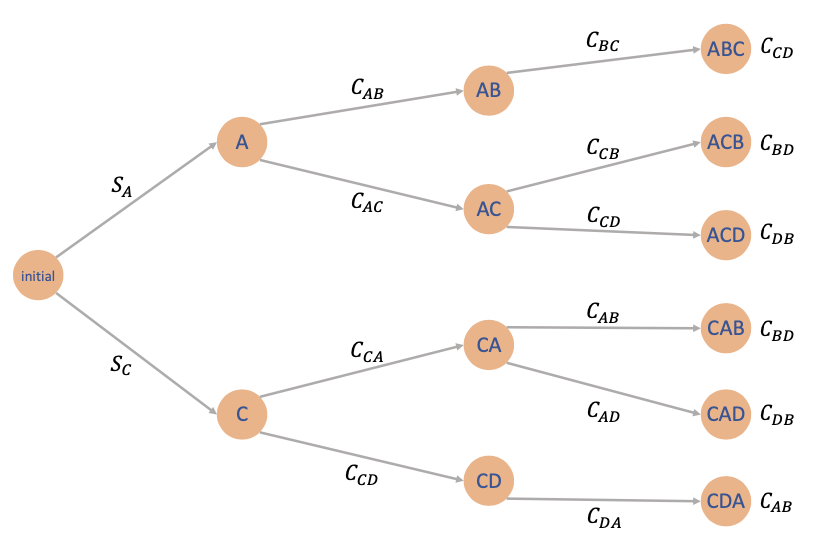
A Deterministic Scheduling Problem

Example
Prof Li ZENG wants to produce luxury headphones that perform better than the bear-pods 3 that he is currently using. To do so, four operations must be performed on a certain machine, and they are denoted by A, B, C, D. Assuming that

1. operation B can only be performed after operation A

2. operation D can only be performed after operation C

Denote

• setup cost Cmn for passing any operation m to n

• initial startup cost SA or SC (can only start with operation A or C)

Solution

• We need to make three decisions (the last is determined by the first three)

• This problem is deterministic (no wk )

• This problem has finite number of states

• Deterministic problems with finite number of states => transition graph

Discrete-State and Finite-State Problems

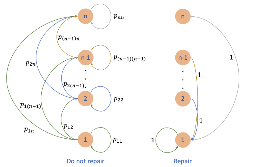
To capture the transition between states, it is often convenient to define the transition probabilities

$$p_{ij}(u,k) = \mathbb{P}(x_{k+1} = j | x_k = i, u_k = u)$$

In the dynamic system, it means that $x_{k+1} = w_k$, where $w_k$ follows a probabilitydistribution which has probabilities $p_{ij}(u,k)$'s.

Example

Consider a problem of N time periods that a machine can be in any one of n states. We denote $g(i)$ as the operating cost per period when the machine is in state i. Assume that

$$g(1) ≤ g(2) ≤ ··· ≤ g(n)$$

That is, a machine in state i works more efficiently than a machine that is in state i + 1. During a period of time, the state of the machine can become worse or stay the same with probability

$$p_{ij} =\mathbb{P}(\text{next state will be } j | \text{current state is } i ) \text{ and } p_{ij} =0,\text{if} j < i.$$

At the start of each period, we can choose

• let the machine operate one more period

• repair the machine and bring it to state 1 (and it will stay there for 1 period) at a cost R

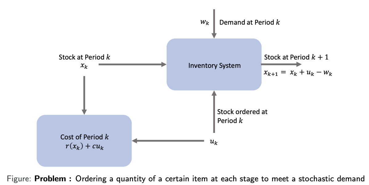
Inventory Control Problem

Ordering a quantity of a certain item at each stage to meet a stochastic demand

• $x_k$: stock available at the beginning of the kth period

• $u_k$: stock ordered and delivered at the beginning of the kth period

• $w_k$: demand during the kth period with given probability distribution

• $r(·)$: penalty/cost for either positive or negative stock

• $c$: cost per unit ordered

Expample: Inventory Control

Suppose $(u_0^{\star}, u_1^\star, \ldots, u_{N-1}^\star)$ is the optimal solution of

$$\min \mathbb{E} \left[ R(x_N) + \sum_{k=0}^{N-1} \left( r(x_k + u_k - w_k) + c \cdot u_k \right) \right]$$

What if:$w_1 = w_2 = \cdots = w_{N-1} = 0$? (recall wi’s are the demands.)

We can do better if we can adjust our decisions to different situations!

Open-Loop and Closed-Loop Control

Open-loop Control

At initial time $k=0$, given initial state $x_0$, find optimal control sequence $(u_0^\star, u_1^\star, \ldots, u_{N-1}^\star)$ minimizing expected total cost:

• Key feature: Subsequent state information is NOT used to adjust control decisions

Closed-loop Control

At each time $k$, make decisions based on current state information $x_k$ (e.g. ordering decision at time $k$):

• Core objective: Find state feedback strategy $\mu_k(\cdot)$ mapping state $x_k$ to control $u_k$

• Decision characteristics:

• Re-optimization at each decision point $k$

• Control rule designed for every possible state value $x_k$

• Computational properties:

• Higher computational cost (requires real-time state mapping)

• Same performance as open-loop when no uncertainty exists

Closed-loop Control

Core Concepts

• Control Law Definition
  Let $\mu_k(\cdot)$ be a function mapping state $x_k$ to control $u_k$:

$$u_k = \mu_k(x_k)$$

• Control Policy
  Define a policy $\pi$ as a sequence of control laws:

$$\pi = {\mu_0, \mu_1, \ldots, \mu_{N-1}}$$

• Policy Cost Function
  Given initial state $x_0$, the expected cost of policy $\pi$ is:

$$J_{\pi}(x_0) = \mathbb{E} \left[ g_N (x_N) + \sum_{k=0}^{N-1} g_k \big( x_k, \mu_k(x_k), w_k \big) \right]$$

Admissible Policy

A policy $\pi = \{\mu_0, \ldots, \mu_{N-1}\}$ is called admissible if and only if:

$$\mu_k(x_k) \in U_k(x_k), \quad \forall x_k \in S_k, \ \forall k = 0,1,\ldots,N-1$$

Meaning at each time $k$ and for every possible state $x_k$, the control $u_k$ must belong to the allowable control set $U_k(x_k)$.

Summary

Definition

Consider a function $J^*$ defined as:

$$J^*(x_0) = \min_{\pi \in \Pi} J^{\pi}(x_0), \quad \forall x_0 \in S_0$$

where:

• $\Pi$: Set of all admissible policies

• $J^{\pi}(x_0)$: Expected cost of policy $\pi$ starting from initial state $x_0$

We call $J^*$ the optimal value function.

Key Properties

1. Global Optimality
   $J^*$ gives the minimum possible expected cost from any initial state $x_0$

2. Policy Independence
   Represents theoretical performance limit, independent of specific policies

3. Benchmarking Role
   Any admissible policy $\pi$ satisfies:

$$J^{\pi}(x_0) \geq J^*(x_0), \quad \forall x_0 \in S_0$$

Computational Significance

• Core Objective of DP: Compute $J^*$ exactly via backward induction

• Control Engineering Application: Measure gap between actual policies and theoretical optimum

The Dynamic Programming Algorithm

Principle of Optimality

Theorem Statement

Let $\pi^* = \{\mu_0^*, \mu_1^*, \ldots, \mu_{N-1}^*\}$ be an optimal policy for the basic problem. Suppose when using $\pi^*$, the system reaches state $x_i$ at time $i$ with positive probability. Consider the subproblem starting from $(x_i, i)$:

$$\min \mathbb{E} \left[ g_N(x_N) + \sum_{k=i}^{N-1} g_k \big( x_k, \mu_k(x_k), w_k \big) \right]$$

Then the truncated policy $\{\mu_i^*, \mu_{i+1}^*, \ldots, \mu_{N-1}^*\}$ is optimal for this subproblem.

Core Implications

1. Heritability of Optimality
   Any tail portion of a globally optimal policy remains optimal for its starting state

2. Time Consistency
   Optimal decisions account for both immediate cost and optimal future state evolution

3. Foundation for Backward Induction
   This principle validates the dynamic programming backward solution approach.

Practical Significance

• Reduces Computational Complexity: Decomposes problem into nested subproblems

• Guarantees Global Optimality: Concatenation of locally optimal decisions yields global optimum

• Enables Real-time Decision Making: Supports receding horizon methods like MPC