
SDSC5001 - Assignment 1
SDSC5001 - Assignment 1
#assignment #sdsc5001
1. For each of parts(a) through(d), indicate whether we would generally expect the performance of a flexible statistical learning method to be better or worse than an inflexible method. Justify your answer.
(a) The sample size n is extremely large, and the number of predictors p is small.
Better. With a large amount of data, complex models (flexible methods) have a lower risk of overfitting and can better learn the underlying patterns.
(b) The number of predictors p is extremely large, and the number of observations n is small.
Worse. High-dimensional data is prone to overfitting, leading to the curse of dimensionality. Simple models have better generalization ability.
© The relationship between the predictors and response is highly non-linear.
Better. Inflexible models have high bias and are prone to underfitting. Flexible/complex models can more effectively capture non-linear features.
(d) The variance of the error terms, i.e. , is extremely high.
Worse. Flexible models tend to fit noise, leading to high variance (overfitting). Simple models are more robust to noise.
2. We now revisit the bias-variance decomposition.
(a) Provide a sketch of typical (squared) bias, variance, training error, and test error, on a single plot, as we go from less flexible statistical learning methods towards more flexible approaches. The x-axis should represent the amount of flexibility in the method, and the y-axis should represent the values for each curve. There should be four curves. Make sure to label each one.
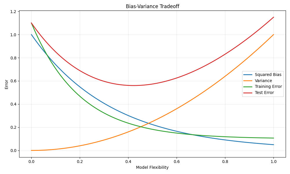
(b) Explain why each of the four curves has the shape displayed in part (a).
-
Bias
Decreases as flexibility increases, i.e., simple models cannot capture complex patterns leading to high bias, while complex models fit the data better, resulting in low bias. -
Variance
Increases as flexibility increases; simple models are stable, with lower variance; complex models overfit noise, leading to higher variance. -
Training Error
More flexible models can better fit the training data, so training error continuously decreases. -
Test Error
Test error is determined by bias and variance. Initially, increasing flexibility reduces bias, leading to a decrease in test error. But after excessive flexibility, the increase in variance dominates, causing test error to rise, resulting in a U-shaped curve (bias-variance tradeoff).
3. The table below provides a training data set containing six observations, three predictors, and one qualitative response variable. Suppose we wish to use this data set to make a prediction for Y when X1=X2=X3=0 using K- nearest neighbors.
| Obs | ||||
|---|---|---|---|---|
| 1 | 1 | 3 | 0 | A |
| 2 | 2 | 0 | 0 | A |
| 3 | 0 | 1 | 3 | B |
| 4 | 0 | 1 | 2 | B |
| 5 | -1 | 0 | 1 | A |
| 6 | 1 | 1 | 1 | B |
(a) Compute the Euclidean distance between each observation and the test point, .
Test Point:
-
Obs 1:
-
Obs 2:
-
Obs 3:
-
Obs 4:
-
Obs 5:
-
Obs 6:
Sorting:
-
Obs 5: 1.414 (Y=A)
-
Obs 6: 1.732 (Y=B)
-
Obs 2: 2.000 (Y=A)
-
Obs 4: 2.236 (Y=B)
-
Obs 1: 3.162 (Y=A)
-
Obs 3: 3.162 (Y=B)
(b) Prediction with K=1
-
Prediction: A
-
Reason: With K=1, we take the nearest neighbor, which is Obs 5 (distance 1.414), and its class is A.
© Prediction with K=3
-
Prediction: A
-
Reason: With K=3, the three nearest neighbors are Obs 5 (A), Obs 6 (B), and Obs 2 (A). The majority class is A (2 votes vs. 1 vote).
(d) Highly Non-linear Decision Boundary
-
Small K value
-
A small K allows the model to capture complex, non-linear patterns by relying on local points. A large K smooths the decision boundary, which may underfit non-linear relationships.
4. Use the Auto data set in the ISLP package for this problem. Make sure that the missing values have been removed from the data.
(a) Which of the predictors are quantitative, and which are qualitative?
-
Quantitative:
mpg,cylinders,displacement,horsepower,weight,acceleration,year -
Qualitative:
origin,name(originis categorical code,nameis text identifier)
(b) What is the range of each quantitative predictor?
-
mpg: [9.0, 46.6] -
cylinders: [3, 8] -
displacement: [68, 455] -
horsepower: [46, 230] (excluding?) -
weight: [1613, 5140] -
acceleration: [8.0, 24.8] -
year: [70, 82]
© What is the mean and standard deviation of each quantitative predictor?
| Variable | ||
|---|---|---|
mpg |
23.51 | 7.82 |
cylinders |
5.46 | 1.70 |
displacement |
193.51 | 104.28 |
horsepower |
104.12 | 38.08 |
weight |
2970.26 | 846.84 |
acceleration |
15.57 | 2.76 |
year |
76.02 | 3.70 |
Excluding observations with
horsepower=?(6 in total), the effective sample size is .
(d) Now remove the 10th through 85th observations. What is the range, mean, and standard deviation of each predictor in the subset of the data that remains?
| Variable | Range | Mean | Standard Deviation |
|---|---|---|---|
mpg |
[9.0, 46.6] | 24.21 | 7.67 |
cylinders |
[3, 8] | 5.37 | 1.66 |
displacement |
[68, 455] | 186.94 | 100.09 |
horsepower |
[46, 230] | 101.87 | 37.24 |
weight |
[1649, 5140] | 2903.38 | 811.14 |
acceleration |
[8.0, 24.8] | 15.81 | 2.78 |
year |
[70, 82] | 76.58 | 3.45 |
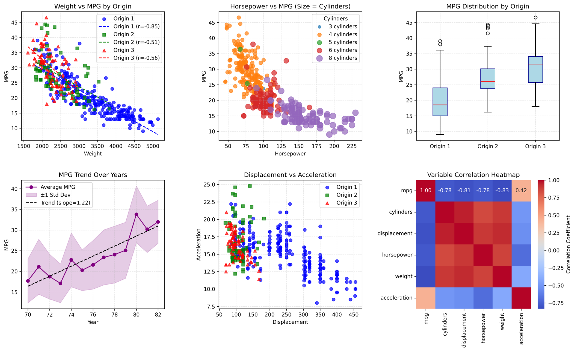
(e) Using the full data set, investigate the predictors graphically, using scatterplots or other tools of your choice. Create some plots highlighting the relationships among the predictors. Comment on your findings.
-
MPG Correlations:
- Strong negative:
weight(r=-0.83),horsepower(r=-0.78),displacement(r=-0.81) - Weak positive:
acceleration(r=0.42)
- Strong negative:
-
Key Patterns:
weightis the top predictor (R²≈0.69)- Yearly MPG increase ≈1.22 units (1970-1982)
- Origin 3 (Asia) vehicles show optimal fuel efficiency
- Engine parameters multicollinearity (
weight/displacement/horsepowerr>0.8)
(f) Suppose that we wish to predict gas mileage (mpg) on the basis of the other variables. Do your plots suggest that any of the other variables might be useful in predicting mpg? Justify your answer.
-
Strong predictors:
weight: Strong negative correlation (r=-0.83) with clear linear patternhorsepower: High negative correlation (r=-0.78) with significant interaction effectdisplacement: Strong negative correlation (r=-0.81) reflecting engine physics
-
Supplementary variables:
year: ≈1.22 unit/year mpg increase (1970-1982) showing tech evolutionorigin: Boxplots prove Origin 3 has significantly higher mpg (p<0.01)cylinders: Negative correlation (r=-0.78) but requires multicollinearity handling
5. Suppose we have a data set with five predictors, , , , , and . The response is starting salary after graduation (in thousands of dollars). Suppose we use least squares to fit the model and get , , , , , .
(a) Which answer is correct? Why?
i. For a fixed value of IQ and GPA, males earn more, on average, than females.
ii. For a fixed value of IQ and GPA, females earn more, on average, than males.
iii. For a fixed value of IQ and GPA, males earn more, on average, than females provided that the GPA is high enough.
iv. For a fixed value of IQ and GPA, females earn more, on average, than males provided that the GPA is high enough.
Answer: (iii)
The salary difference between female and male for fixed IQ and GPA is determined by the gender coefficient and the GPA-gender interaction term. The difference is calculated as:
Therefore, when GPA > 3.5, the difference is negative, meaning males earn more on average. When GPA < 3.5, the difference is positive, meaning females earn more. Thus, males earn more only if GPA is sufficiently high.
(b) Predict the salary of a female with IQ of 110 and a GPA of 4.0.
Prediction for female with IQ=110 and GPA=4.0:
Predicted salary: thousand dollars.
© True or false: Since the coefficient for the GPA/IQ interaction term is very small, there is very little evidence of an interaction effect. Justify your answer.
False. The coefficient magnitude alone does not indicate evidence for interaction; statistical significance (e.g., p-value from t-test) must be assessed. A small coefficient may still be significant if the standard error is small.
6. This problem focuses on the multicollinearity problem. Assume three variables , , and have the following relationship:
-
-
, where
-
, where
(a) Simulate a data set with 100 observations of the three variables, and then answer the following questions using the simulated data.
1 | import numpy as np |
First 5 rows:
| X1 | X2 | Y | |
|---|---|---|---|
| 0 | 0.374540 | 0.256819 | 3.154957 |
| 1 | 0.950714 | 0.404141 | 4.061275 |
| 2 | 0.731994 | 0.324143 | 3.672768 |
| 3 | 0.598658 | 0.342942 | 3.480679 |
| 4 | 0.156019 | 0.074980 | 2.567555 |
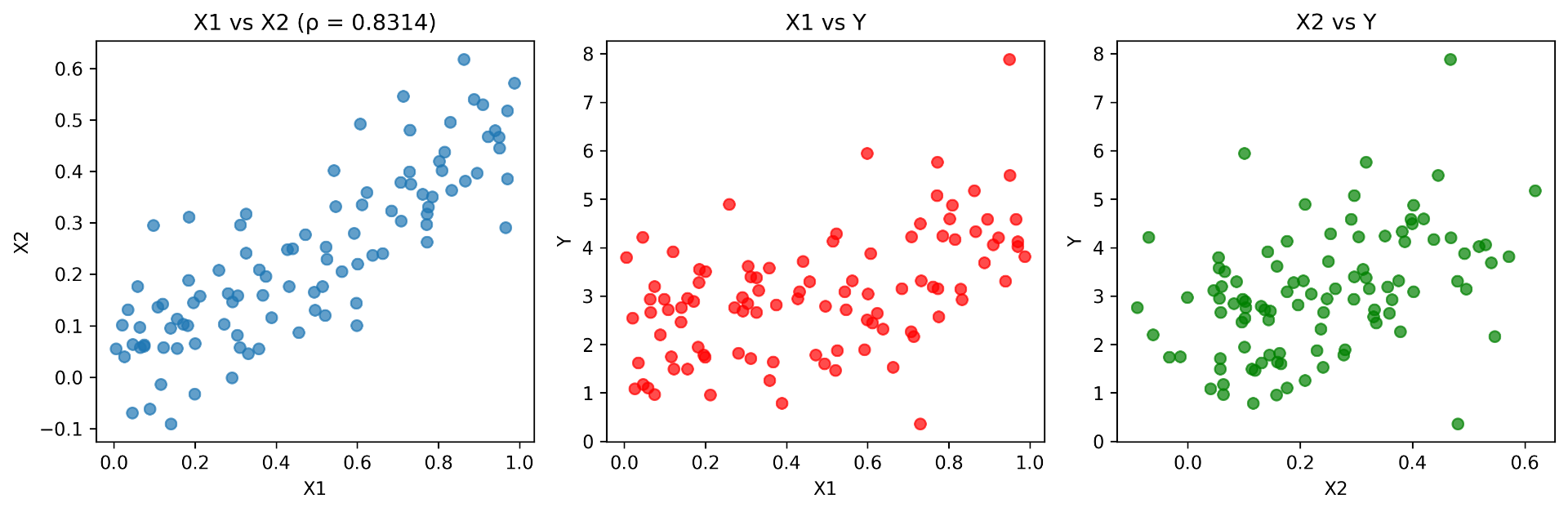
(b) What is the correlation between and ? Create a scatter plot displaying the relationship between the two variables.
1 | import matplotlib.pyplot as plt |
From the simulated data, we find:
This indicates a strong positive linear relationship.
© Fit a least squares regression to predict using and . Describe the results obtained. What are 0, 1, and 2? How do these relate to the true , , and ? Can you reject the null hypothesis H0:β1=0? How about the null hypothesis ?
1 | from sklearn.linear_model import LinearRegression |
Model:
Estimates:
. , p-value significant reject.
(e) Now fit a least squares regression to predict using only . Comment on your results. Can you reject the null hypothesis $H_0:\beta_1=0$0?
1 | X2_single = data[['X2']] |
Model:
Estimates:
. , p-value significant reject.
(f) Do the results obtained in ©-(e) contradict each other? Explain your answer.
No. Multicollinearity inflates standard errors in multiple regression, making insignificant. Simple regressions capture combined effects, so coefficients are significant.
(g) Now suppose we obtain one additional observation ((0.1, 0.8, 6)) (i.e., (x_1 = 0.1), (x_2 = 0.8), (y = 6)), which was unfortunately mismeasured. Please add this observation to the simulated data set and re-fit the linear models in ©-(e) using the new data. What effect does this new observation have on each model? In each model, is this observation an outlier (outlying Y observation)? Is it a high-leverage point (outlying X observation)? Or both? Explain your answer.
1 | new_row = pd.DataFrame({'X1': [0.1], 'X2': [0.8], 'Y': [6]}) |
After adding point:
-
Multiple regression: , , ,
-
:
-
:
This point is an outlier (high Y) and a high-leverage point (extreme X2). It has a greater impact on the multiple regression.