SDSC5001 Course 3-Overview of Statistical Machine Learning

#sdsc5001

English / 中文

---

Comparison of Terminology Between Statistics and Machine Learning

Statistics	Machine Learning
Classification/Regression Clustering Classification/Regression with missing responses (Nonlinear) Dimensionality Reduction	Supervised Learning Unsupervised Learning Semi-supervised Learning Manifold Learning
Covariates/Response Variables Sample/Population Statistical Model Misclassification/Prediction Error	Features/Outcome Training Set/Test Set Learner Generalization Error
Multinomial Logistic Function Truncated Linear Function	Softmax Function ReLU (Rectified Linear Unit)

Key Note: The two fields use different terminology to describe similar concepts, but the core ideas are interconnected. For example, “covariates” in statistics correspond to “features” in machine learning.

---

Practical Application Cases

Wage Prediction Case

Task: Understand the relationship between employee wages and multiple factors

Data Source: Dataset collected based on male employees in the Atlantic region of the United States

Spam Detection Case

Task: Build a filter that can automatically detect spam emails

Data Representation:

Observation	make%	address%	…	Total Capital Letters	Is Spam
1	0	0.64	…	278	1(Yes)
2	0.21	0.28	…	1028	1(Yes)
3	0	0	…	7	0(No)
…	…	…	…	…	…
4600	0.3	0	…	78	0(No)
4601	0	0	…	40	0(No)

Dataset Characteristics:

• 4601 emails, 2 categories

• 57 term frequency features

• Simple classification function: $I(\text{Capital\_total} > 100)$, where $I(\cdot)$ is the indicator function

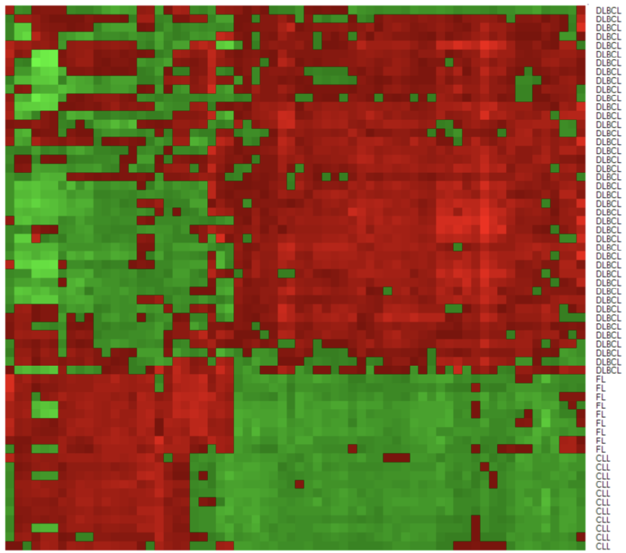
Gene Microarray Case

Task: Automatically diagnose cancer based on patient genotypes
Data Characteristics:

• 4026 gene expression profiles

• 62 patients, 3 types of adult lymphoid malignancies

• 66 “carefully” selected genes

---

Basic Notation

Training samples: $\left(x_{i}, y_{i}\right)_{i=1}^{n}$

• $x_{i}$: input, feature vector, predictor variable, independent variable, $x_i \in \mathbb{R}^p$

• $y_i$: output, response variable, dependent variable, scalar (can also be a real vector)

Data generation model:

$$Y = f(X) + \epsilon$$

• $f$: unknown function, represents systematic information about Y provided by X

• $\epsilon$: random error term, satisfying:

  • Mean zero: $\mathbb{E}(\epsilon)=0$
  • Independent of X

Reasons for the error term $\epsilon$:

1. Unmeasured factors

2. Measurement error

3. Intrinsic randomness

---

Estimation Methods

Parametric Models

• Linear/Polynomial regression models

• Generalized linear regression models

• Fisher discriminant analysis

• Logistic regression

• Deep learning

Nonparametric Models

• Local smoothing

• Smoothing splines

• Classification and regression trees, random forests, boosting methods

• Support vector machines

---

Prediction and Inference

Prediction

Based on the estimated function $\hat{f}$, predict the response for new X:

$$\widehat{Y} = \hat{f}(X)$$

Prediction error decomposition:

$$\mathbb{E}(\widehat{Y}-Y)^{2} = \underbrace{\mathbb{E}(\hat{f}(X)-f(X))^{2}}_{\text{Reducible Error}} + \underbrace{\operatorname{var}(\epsilon)}_{\text{Irreducible Error}}$$

• Reducible Error: Can be reduced by improving learning techniques

• Irreducible Error: Cannot be eliminated due to $\epsilon$ being unpredictable by X

Inference

Goal: Understand how Y is affected by X

• Which predictors are associated with Y?

• How is Y related to each predictor?

• How does Y change when intervening on certain predictors?

Balance between Prediction and Inference:

• Simple models (e.g., linear models): High interpretability but possibly lower prediction accuracy

• Complex nonlinear models: High prediction accuracy but poor interpretability

---

Classification Problems

Classification differs slightly from regression:

$$P(Y=k \mid X)=f_{k}(X); \quad k=1,\ldots, K$$

Classification decision function:

$$\hat{\phi}(X) = \underset{k}{\operatorname{argmax}} \hat{f}_{k}(X)$$

Misclassification error:

$$P(Y \neq \hat{\phi}(X)) = \mathbb{E}(I(Y \neq \hat{\phi}(X)))$$

---

Example: Binary Classification Toy Problem

Problem Description: Simulate 200 points from an unknown distribution, two classes {blue, orange} with 100 each, build a prediction rule

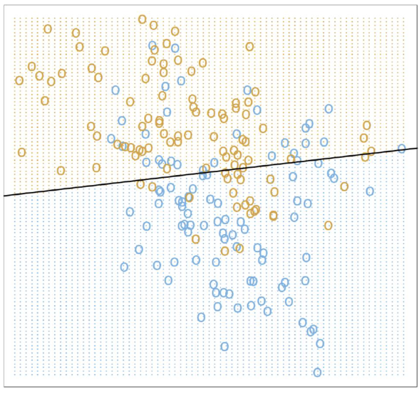
Model 1: Linear Regression

Encoding: $Y=1$ (orange), $Y=0$ (blue)

Model form:

$$Y = \beta_0 + \sum_{j=1}^p X_j\beta_j = X\beta$$

Parameter estimation (least squares):

$$\hat{\beta} = \left(X^{T} X\right)^{-1} X^{T} y$$

Classification decision function:

$$\hat{\phi}(X) = I\left(X^T\hat{\beta} > 0.5\right)$$

Model 2: K-Nearest Neighbors (K-NN)

Prediction based on neighbors:

$$\hat{y}(X) = \frac{1}{k}\sum_{i=1}^n y_i I\left(x_i \in N_k(X)\right)$$

where $N_k(X)$ is the neighborhood of X containing exactly k neighbors

Classification decision function (majority vote):

$$\widehat{\phi}(X) = I(\widehat{y}(X) > 0.5)$$

Model Complexity Comparison:

• Linear regression: Uses 3 parameters

• K-NN classifier: Uses $n/k$ effective parameters

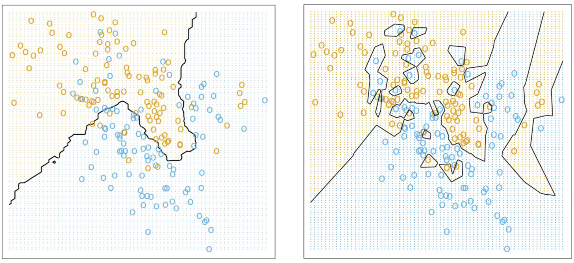
Comparison of 15-NN and 1-NN classification results

---

Regression Model Evaluation

Mean Squared Error (MSE) and Its Minimization

Definition of Mean Squared Error (MSE)

For regression problems where $Y \in \mathbb{R}$ and $X \in \mathbb{R}^p$, the accuracy of a function $f$ can be measured by the Mean Squared Error (MSE). MSE is defined as:

$$\operatorname{MSE}(f) = \mathbb{E}\left[(Y - f(X))^2\right]$$

where the expectation $\mathbb{E}$ is taken over the joint distribution of $X$ and $Y$. MSE measures the average squared difference between the predicted value $f(X)$ and the true value $Y$, and is an important metric for evaluating the performance of predictive models.

Intuitive Explanation: A smaller MSE indicates more accurate predictions by the model. It penalizes larger errors more severely (due to the squared term), making it sensitive to outliers.

Minimizer of MSE

Theory shows that the minimizer of MSE is the conditional expectation function:

$$f^*(X) = \mathbb{E}[Y \mid X]$$

This means that MSE reaches its minimum when $f(X)$ equals the conditional expectation of $Y$ given $X$. This result comes from the properties of conditional expectation in probability theory: $\mathbb{E}[Y \mid X]$ is the best predictor of $Y$ given $X$ (in the sense of minimizing squared error).

Brief derivation:

By expanding MSE:

$$\mathbb{E}[(Y - f(X))^2] = \mathbb{E}[(Y - \mathbb{E}[Y|X] + \mathbb{E}[Y|X] - f(X))^2]$$

Using properties of conditional expectation, it can be shown that:

$$\mathbb{E}[(Y - f(X))^2] = \mathbb{E}[(Y - \mathbb{E}[Y|X])^2] + \mathbb{E}[(\mathbb{E}[Y|X] - f(X))^2]$$

Since the first term is constant (independent of $f$), minimizing MSE is equivalent to minimizing the second term, which is zero when $f(X) = \mathbb{E}[Y|X]$.

Training Error

In practice, the joint distribution $(X, Y)$ is unknown, so we cannot directly compute the theoretical MSE. Instead, we approximate the Mean Squared Error (MSE) based on a sample dataset $\{(x_i, y_i)\}_{i=1}^n$.

$$\widehat{\operatorname{MSE}}(f) = \frac{1}{n} \sum_{i=1}^{n} (y_i - f(x_i))^2$$

This is called the empirical risk or training error. However, note that:

• This estimate is an approximation of the theoretical MSE but may be biased, especially if the model overfits the training data.

• Tends to underestimate the true MSE; complex models may achieve very small training errors

Test Error

Using independent test samples $\left(x_{0 i}, y_{0 i}\right)_{i=1}^{m}$:

$$\frac{1}{m}\sum_{i=1}^{m}\left(y_{0 i}-\hat{f}\left(x_{0 i}\right)\right)^{2}$$

Advantage: Closer to the true MSE, simulates future observations to be predicted

---

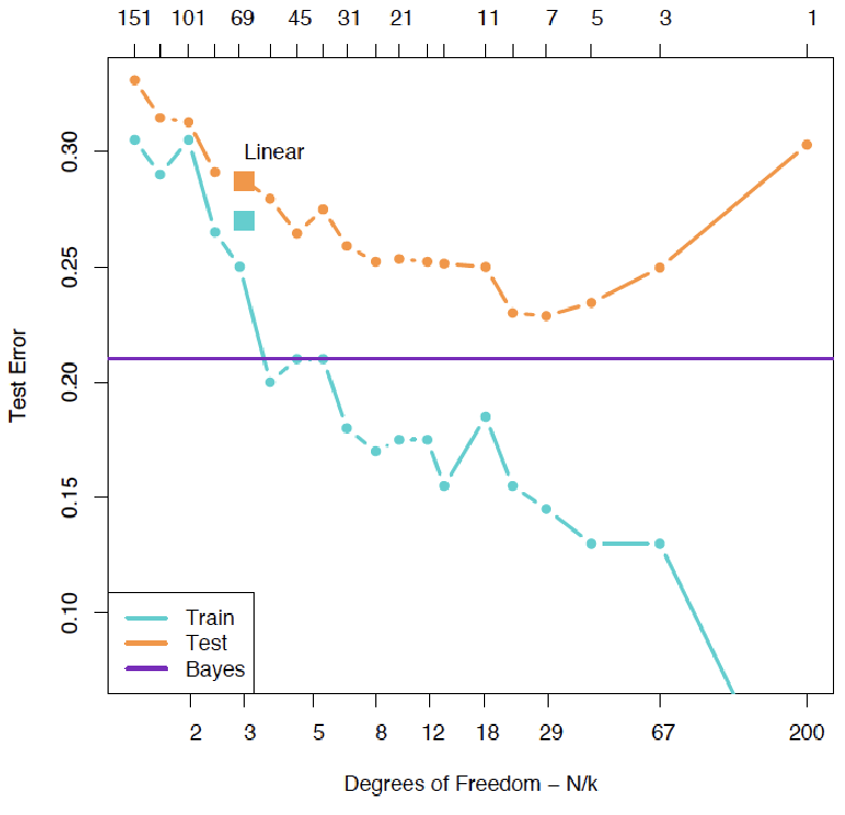
Bias-Variance Decomposition

U-Shaped Curve of Test Error

The test error changes with model complexity in a typical U-shaped curve, resulting from the interaction of two competing quantities:

$$\begin{align*} \mathbb{E}[(Y-\hat{f}(X))^2] = & \mathbb{E}[(\hat{f}(X)-f(X))^2] + \operatorname{var}(\varepsilon) \\ = & [\operatorname{Bias}(\hat{f}(X))]^2 + \operatorname{var}(\hat{f}(X)) + \operatorname{var}(\varepsilon) \end{align*}$$

Key Note: This decomposition reveals three sources of prediction error: bias, variance, and irreducible error.

Bias Term

$$\operatorname{Bias}(\hat{f}(X)) = \mathbb{E}[\hat{f}(X)] - f(X)$$

• Definition: The difference between the expectation of the estimate $\hat{f}(X)$ and the true function $f(X)$

• Meaning: Systematic error introduced by approximating $f$ with $\hat{f}$

• Characteristic: Reflects the model’s fitting capability

Variance Term

$$\operatorname{var}(\hat{f}(X)) = \mathbb{E}[(\hat{f}(X)-\mathbb{E}[\hat{f}(X)])^2]$$

• Definition: The degree of fluctuation of the estimate $\hat{f}(X)$ around its expectation

• Meaning: How much $\hat{f}$ would change if estimated using different training sets

• Characteristic: Reflects the model’s sensitivity to changes in training data

Irreducible Error

$$\operatorname{var}(\varepsilon)$$

• Definition: Variance of the random error term $\varepsilon$

• Meaning: Error due to intrinsic randomness in the data, cannot be reduced by improving the model

• Characteristic: Sets a theoretical lower bound for prediction error

Bias-Variance Trade-off

As model complexity increases:

• Bias decreases: Complex models can better fit complex patterns in the data

• Variance increases: Complex models are more sensitive to noise in the training data

This trade-off leads to the U-shaped curve of test error:

• Simple models: High bias, low variance (underfitting)

• Complex models: Low bias, high variance (overfitting)

• Optimal model: Balances bias and variance

Example: In linear regression, adding polynomial features can reduce bias but increase variance; regularization (e.g., ridge regression) can reduce variance but may slightly increase bias.

---

Classification Model Evaluation

Misclassification Error

For classification problems where $Y \in \{1, \ldots, K\}$ and $X \in \mathbb{R}^p$, the accuracy of a function $f$ can be measured by the misclassification error:

$$\operatorname{MCE}(f) = \mathbb{E}[I(Y \neq f(X))]$$

where the expectation $\mathbb{E}$ is taken over the joint distribution of $X$ and $Y$, and $I(\cdot)$ is the indicator function.

Intuitive Explanation: Misclassification error measures the probability that the model makes an incorrect classification, and is the most direct performance metric for classification problems.

Bayes Rule

The minimizer of misclassification error must satisfy:

$$f^{*}(X) = \underset{k}{\arg\max} P(Y=k \mid X)$$

This is called the Bayes rule or Bayes classifier, and is the optimal classification decision given the features $X$.

Derivation Note:
For any classification rule $\phi(X)$, its conditional misclassification error is:

$$P(Y \neq \phi(X) \mid X = x) = 1 - P(Y = \phi(x) \mid X = x)$$

To minimize this probability, choose $\phi(x)$ such that $P(Y = \phi(x) \mid X = x)$ is maximized, i.e., choose the class with the highest posterior probability.

Training Error and Test Error

Training Error

Given training samples $\{(x_i, y_i)\}_{i=1}^n$ and an estimated function $\hat{f}$, its training error is:

$$\frac{1}{n} \sum_{i=1}^{n} I(y_i \neq \hat{f}(x_i))$$

Characteristic: Measures the model’s performance on training data, but may underestimate the true misclassification error.

Test Error

If there are test samples $\{(x_{0i}, y_{0i})\}_{i=1}^m$, the test error of $\hat{f}$ is:

$$\frac{1}{m} \sum_{i=1}^{m} I(y_{0i} \neq \hat{f}(x_{0i}))$$

Characteristic: Provides an unbiased estimate of the model’s performance on new data, and is the gold standard for evaluating model generalization ability.

---

Cross-Validation Methods

Validation Set Method

Advantages: Simple idea, easy to implement
Disadvantages:

• Validation MSE can be highly variable

• Uses only part of the observations to fit the model, performance may degrade

Leave-One-Out Cross-Validation (LOOCV)

Steps:

1. Split the dataset of size n into: training set (n-1) and validation set (1)

2. Fit the model using the training set

3. Validate the model using the validation set, compute MSE

4. Repeat n times

5. Compute the average MSE

Advantages:

• Low bias (uses n-1 observations)

• Produces less variable MSE

Disadvantages: Computationally intensive

K-Fold Cross-Validation

Steps:

1. Divide the training samples into $A_{1},\ldots, A_{K}$ (usually K=5 or 10)

2. For each k, fit the model $\hat{f}^{-k}(x)$ using all data except $A_k$

3. Compute the prediction error on $A_k$:

   $$E_{k}(\hat{f}) = \sum_{i\in A_{k}} L\left(y_{i},\hat{f}^{-k}\left(x_{i}\right)\right)^{2}$$

4. Compute the CV error:

   $$CV(\hat{f}) = \frac{1}{n}\sum_{k=1}^{K} E_{k}(\hat{f})$$

Comparison of Cross-Validation Methods

Based on comparison of three simulated examples:

• Blue: Test error

• Black: LOOCV

• Orange: 10-fold CV

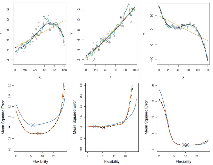
Conclusions:

• LOOCV has lower bias than K-fold CV (when $K < n$)

• LOOCV has higher variance than K-fold CV (when $K < n$)

• In practice, K-fold CV with K=5 or 10 is commonly used

• Empirical evidence shows that K-fold CV provides reasonable estimates of test error