SDSC5001 Course 4-Linear Regression

#sdsc5001

English / 中文

Simple Linear Regression

Basic Setup

Given data $\left(x_{1}, y_{1}\right),\ldots,\left(x_{n}, y_{n}\right)$, where:

• $x_{i} \in \mathbb{R}$ is the predictor variable (independent variable, input, feature)

• $y_{i} \in \mathbb{R}$ is the response variable (dependent variable, output, outcome)

The regression function is expressed as:

$$y = f(x) + \varepsilon$$

The linear regression model assumes:

$$f(x) = \beta_0 + \beta_1 x$$

This is usually considered an approximation of the true relationship.

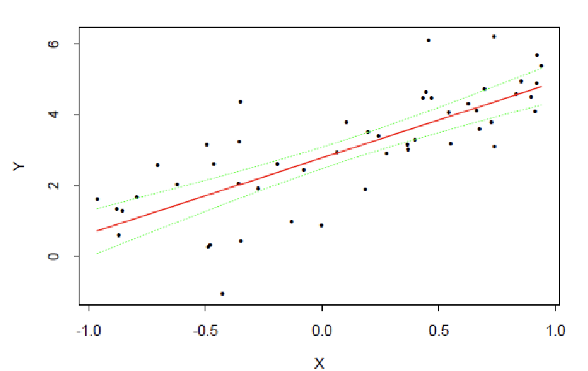
Example (Attachment Page 2): A simple toy example showing data points and linear fit.

Least Squares Fitting

Parameters are estimated by minimizing the residual sum of squares:

$$\min_{\beta_0, \beta_1} \sum_{i=1}^{n} (y_i - (\beta_0 + \beta_1 x_i))^2$$

The solutions are:

$$\begin{aligned} &\hat{\beta}_1 = \frac{\sum_{i=1}^{n} (x_i - \bar{x})(y_i - \bar{y})}{\sum_{i=1}^{n} (x_i - \bar{x})^2}\\ &\hat{\beta}_0 = \bar{y} - \hat{\beta}_1 \bar{x} \end{aligned}$$

Where:

• $\hat{y}_i = \hat{\beta}_0 + \hat{\beta}_1 x_i$ is the fitted value

• $e_i = y_i - \hat{y}_i$ is the residual

Parameter Estimation and Statistical Inference

Model Assumptions

Assume the data generating process is:

$$Y_i = \beta_0 + \beta_1 x_i + \varepsilon_i$$

where $\varepsilon_i$ are i.i.d. $N(0, \sigma^2)$

Under these assumptions, it can be proven:

• $\hat{\beta}_0$ and $\hat{\beta}_1$ are unbiased estimators of $\beta_0$ and $\beta_1$

  $$\hat{\beta}_1 \sim N\left(\beta_1,\frac{\sigma^2}{\sum_i(x_i - \bar{x})^2}\right)$$

• $\hat{\beta}_1$ has the smallest variance among all unbiased linear estimators (BLUE estimator)

  $$\hat{\beta}_0 \sim N\left(\beta_0,\left\{\frac{1}{n} + \frac{\bar{x}^2}{\sum_i(x_i - \bar{x})^2}\right\}\sigma^2\right)$$

Derivation of Unbiasedness

To prove $\hat{\beta}_1$ is unbiased, we first write the formula for $\hat{\beta}_1$:

$$\hat{\beta}_1 = \frac{\sum_{i=1}^n (x_i - \bar{x})(y_i - \bar{y})}{\sum_{i=1}^n (x_i - \bar{x})^2}$$

where $\bar{x} = \frac{1}{n} \sum x_i$ and $\bar{y} = \frac{1}{n} \sum y_i$.

Substitute $y_i = \beta_0 + \beta_1 x_i + \varepsilon_i$, and note that $\bar{y} = \beta_0 + \beta_1 \bar{x} + \bar{\varepsilon}$, where $\bar{\varepsilon} = \frac{1}{n} \sum \varepsilon_i$.

After algebraic simplification (specific steps omitted), we get:

$$\hat{\beta}_1 = \beta_1 + \frac{\sum (x_i - \bar{x}) \varepsilon_i}{\sum (x_i - \bar{x})^2}$$

Taking expectation:

$$E[\hat{\beta}_1] = E\left[\beta_1 + \frac{\sum (x_i - \bar{x}) \varepsilon_i}{\sum (x_i - \bar{x})^2}\right] = \beta_1 + \frac{\sum (x_i - \bar{x}) E[\varepsilon_i]}{\sum (x_i - \bar{x})^2} = \beta_1$$

because $E[\varepsilon_i] = 0$. Therefore, $\hat{\beta}_1$ is unbiased.

Similarly, for $\hat{\beta}_0 = \bar{y} - \hat{\beta}_1 \bar{x}$, taking expectation:

$$E[\hat{\beta}_0] = E[\bar{y}] - \bar{x} E[\hat{\beta}_1] = (\beta_0 + \beta_1 \bar{x}) - \bar{x} \beta_1 = \beta_0$$

So $\hat{\beta}_0$ is also unbiased.

Practical Significance: Unbiasedness means that over many repeated samples, the average of the estimates will be close to the true parameter value, increasing the reliability of the estimation.

Derivation of BLUE Property (Gauss-Markov Theorem)

The Gauss-Markov theorem states that in the linear regression model, if the error terms have zero mean, constant variance, and are uncorrelated, then the least squares estimator $\hat{\beta}_1$ has the smallest variance among all linear unbiased estimators.

Consider any linear unbiased estimator $b_1 = \sum_{i} c_i y_i$, where $c_i$ are constants. Unbiasedness requires $E[b_1] = \beta_1$, which implies $\sum c_i = 0$ and $\sum c_i x_i = 1$ (by substituting the expression for $y_i$).

The variance is:

$$\text{Var}(b_1) = \text{Var}\left(\sum c_i y_i\right) = \sum c_i^2 \text{Var}(y_i) = \sigma^2 \sum c_i^2$$

because $\text{Var}(y_i) = \sigma^2$.

The variance of the least squares estimator $\hat{\beta}_1$ is:

$$\text{Var}(\hat{\beta}_1) = \frac{\sigma^2}{\sum (x_i - \bar{x})^2}$$

Through an optimization problem, it can be shown that for any other linear unbiased estimator $b_1$, $\text{Var}(b_1) \geq \text{Var}(\hat{\beta}_1)$. This demonstrates the minimum variance property of $\hat{\beta}_1$.

Practical Significance: The BLUE property means the OLS estimator is the most precise (minimum variance), thus more efficient in statistical inference, e.g., producing narrower confidence intervals.

Illustrative Example

Suppose we have a simple dataset: house area ($x_i$) and house price ($y_i$). The model is $y_i = \beta_0 + \beta_1 x_i + \varepsilon_i$.

• $\beta_0$ might represent the base price when the area is 0 (though this may not be meaningful in practice, so it is often considered a model offset).

• $\beta_1$ represents the average increase in price per additional square meter.

• Unbiasedness: If we collect data multiple times and compute $\hat{\beta}_1$, its average will be close to the true $\beta_1$.

• BLUE: If we use other linear methods (e.g., weighted least squares) but choose weights inappropriately, the variance might be larger, making the estimation less stable than OLS.

Confidence Intervals

$\sigma^2$ can be estimated unbiasedly by MSE:

$$\hat{\sigma}^2 = \text{MSE} = \frac{\sum_{i=1}^{n} (y_i - \hat{y}_i)^2}{n-2}$$

Based on Cochran’s theorem, the confidence intervals for $\hat{\beta}_0$ and $\hat{\beta}_1$ are:

$$\hat{\beta}_j \pm t\left(\frac{\alpha}{2}, n-2\right) \cdot \text{se}(\hat{\beta}_j), \quad j=0,1$$

Symbol Definitions and Interpretations

• $\sigma^2$: Variance of the error term, representing the variation in the data not accounted for by the model. It is an unknown constant parameter.

• $\hat{\sigma}^2$ or MSE: Mean Squared Error, an unbiased estimator of $\sigma^2$. Calculated as $\hat{\sigma}^2 = \text{MSE} = \frac{\sum_{i=1}^{n} (y_i - \hat{y}_i)^2}{n-2}$, where $n$ is the sample size, and $n-2$ is the degrees of freedom (because two parameters $\beta_0$ and $\beta_1$ are estimated). MSE measures the average squared prediction error of the model.

• $\text{se}(\hat{\beta}_j)$: Standard error of the estimator $\hat{\beta}_j$, representing the standard deviation of the sampling distribution of $\hat{\beta}_j$. For simple linear regression:

  • $\text{se}(\hat{\beta}_0) = \sqrt{\text{MSE} \cdot \left( \frac{1}{n} + \frac{\bar{x}^2}{\sum_{i=1}^{n} (x_i - \bar{x})^2} \right)}$
  • $\text{se}(\hat{\beta}_1) = \sqrt{\frac{\text{MSE}}{\sum_{i=1}^{n} (x_i - \bar{x})^2}}$

• $t\left(\frac{\alpha}{2}, n-2\right)$: The upper $\alpha/2$ quantile of the t-distribution, where $\alpha$ is the significance level (e.g., 95% confidence level corresponds to $\alpha=0.05$), and $n-2$ is the degrees of freedom. The t-distribution is used instead of the normal distribution to construct confidence intervals when the population variance is unknown.

Derivation Principle of Confidence Intervals

The derivation of confidence intervals is based on the following steps:

1. Sampling Distribution: Under the model assumptions (error terms $\varepsilon_i \sim N(0, \sigma^2)$ and independent), the least squares estimators $\hat{\beta}_j$ follow a normal distribution:

   $$\hat{\beta}_j \sim N\left(\beta_j, \text{Var}(\hat{\beta}_j)\right)$$

   where $\text{Var}(\hat{\beta}_j)$ is the variance, depending on $\sigma^2$.

2. Variance Estimation: Since $\sigma^2$ is unknown, we use MSE to estimate it. Cochran’s theorem (or related theorems) ensures:

   • $\hat{\sigma}^2 = \text{MSE}$ is independent of $\hat{\beta}_j$.
   • $\frac{(n-2) \text{MSE}}{\sigma^2} \sim \chi^2(n-2)$, i.e., follows a chi-square distribution with $n-2$ degrees of freedom.

3. t-statistic: Standardizing $\hat{\beta}_j$ gives the t-statistic:

   $$t = \frac{\hat{\beta}_j - \beta_j}{\text{se}(\hat{\beta}_j)} \sim t(n-2)$$

   This is because:

   $$t = \frac{\hat{\beta}_j - \beta_j}{\sqrt{\text{Var}(\hat{\beta}_j)}} \bigg/ \sqrt{\frac{\text{MSE}}{\sigma^2}} = \frac{N(0,1)}{\sqrt{\chi^2_{n-2} / (n-2)}}$$

   which is exactly the definition of the t-distribution.

4. Confidence Interval: Based on the properties of the t-distribution:

   $$P\left( -t_{\alpha/2, n-2} \leq \frac{\hat{\beta}_j - \beta_j}{\text{se}(\hat{\beta}_j)} \leq t_{\alpha/2, n-2} \right) = 1 - \alpha$$

   Rearranging the inequality gives the confidence interval:

   $$\hat{\beta}_j \pm t_{\alpha/2, n-2} \cdot \text{se}(\hat{\beta}_j)$$

   This means we are $1-\alpha$ confident that the true parameter $\beta_j$ lies within this interval.

Practical Significance and Interpretation

Confidence intervals provide a measure of uncertainty for parameter estimates. For example, for a 95% confidence interval for $\beta_1$:

• Interpretation: If we repeatedly sample many times and compute a confidence interval each time, about 95% of these intervals will contain the true $\beta_1$.

• Application: If the confidence interval includes zero, it may indicate that the predictor variable has no significant effect on the response variable (but needs hypothesis testing confirmation). The width of the interval reflects the precision of the estimate: a narrower interval indicates higher precision.

• Example: In a house price prediction model, if $\beta_1$ represents the effect of area on price, and its 95% confidence interval is [100, 200], we can say “we are 95% confident that for each additional square meter, the house price increases by an average of 100 to 200 units.”

Illustrative Example

Suppose we have a simple linear regression model predicting test scores ($y$) based on study time ($x$). Sample size $n=20$, calculations give:

• $\hat{\beta}_1 = 5$ (each additional hour of study time increases the score by 5 points on average)

• $\text{se}(\hat{\beta}_1) = 0.8$

• $\text{MSE} = 10$, degrees of freedom $n-2=18$

• For a 95% confidence interval, $\alpha=0.05$, from the t-distribution table $t_{0.025, 18} \approx 2.101$

Then the confidence interval for $\beta_1$ is:

$$5 \pm 2.101 \times 0.8 = [3.32, 6.68]$$

This means we are 95% confident that the true effect of study time is between 3.32 and 6.68 points.

Hypothesis Testing

Test $H_0: \beta_1 = 0$ vs $H_1: \beta_1 \neq 0$:

$$t_1^* = \frac{\hat{\beta}_1}{\text{se}(\hat{\beta}_1)} \sim t_{n-2}$$

If $|t_1^*| > t\left(\frac{\alpha}{2}, n-2\right)$, reject $H_0$

Example: Fitted line and confidence band

Multiple Linear Regression

Model Setup

$$y_i = \beta_0 + \beta_1 x_{i1} + \cdots + \beta_p x_{ip} + \varepsilon_i$$

Matrix form:

$$\mathbf{y} = \mathbf{X}\boldsymbol{\beta} + \boldsymbol{\varepsilon}$$

Where:

• $\mathbf{y}$ is the $n \times 1$ response vector

• $\mathbf{X}$ is the $n \times (p+1)$ design matrix (first column is 1s)

• $\boldsymbol{\beta}$ is the $(p+1) \times 1$ parameter vector

---

Least Squares Estimation

Objective Function

The goal of least squares is to minimize the residual sum of squares:

$$\begin{aligned} \hat{\beta} & = \argmin_{\boldsymbol{\beta}} \sum_{i=1}^{n} \left(y_i - \beta_0 - \sum_{j=1}^{p} \beta_j x_{ji}\right)^2 \\ & = \argmin_{\boldsymbol{\beta}} (\mathbf{y} - \mathbf{X}\boldsymbol{\beta})^\top(\mathbf{y} - \mathbf{X}\boldsymbol{\beta}) \end{aligned}$$

Formula Meaning: The left side is the summation form of the residual sum of squares, the right side is the matrix form. $\mathbf{y}$ is the response vector, $\mathbf{X}$ is the design matrix, $\boldsymbol{\beta}$ is the parameter vector to be estimated.

Least Squares Solution

Solving the above optimization problem gives the parameter estimator:

$$\hat{\boldsymbol{\beta}} = (\mathbf{X}^\top\mathbf{X})^{-1}\mathbf{X}^\top\mathbf{y}$$

Statistical Properties:

• Expectation: $\mathbb{E}[\hat{\boldsymbol{\beta}}] = \boldsymbol{\beta}$ (unbiased estimator)
• Covariance matrix: $\text{cov}(\hat{\boldsymbol{\beta}}) = \sigma^2 (\mathbf{X}^\top\mathbf{X})^{-1}$

Fitted Values and Hat Matrix

Fitted Value Calculation

Using the parameter estimator to get fitted values:

$$\hat{\mathbf{y}} = \mathbf{X}\hat{\boldsymbol{\beta}} = \mathbf{X}(\mathbf{X}^\top\mathbf{X})^{-1}\mathbf{X}^\top\mathbf{y} = \mathbf{H}\mathbf{y}$$

where $\mathbf{H} = \mathbf{X}(\mathbf{X}^\top\mathbf{X})^{-1}\mathbf{X}^\top$ is called the hat matrix.

Hat Matrix Properties:

• $\mathbf{H}$ is a symmetric idempotent matrix ($\mathbf{H}^2 = \mathbf{H}$)
• Trace $\text{tr}(\mathbf{H}) = p + 1$ (number of parameters)
• Projects the response vector $\mathbf{y}$ onto the column space of the design matrix

Statistical Properties of Fitted Values

$$\mathbb{E}[\hat{\mathbf{y}}] = \mathbf{X}\boldsymbol{\beta}\\ \text{cov}(\hat{\mathbf{y}}) = \sigma^2\mathbf{H}$$

Geometric Interpretation: The fitted values $\hat{\mathbf{y}}$ are the orthogonal projection of $\mathbf{y}$ onto the column space of the design matrix.

Residual Properties Analysis

Residual Definition and Expression

The residual vector is defined as the difference between observed and fitted values:

$$\mathbf{e} = \mathbf{y} - \hat{\mathbf{y}} = (\mathbf{I} - \mathbf{H})\mathbf{y}$$

Statistical Properties of Residuals

$$\mathbb{E}[\mathbf{e}] = \mathbf{0}\\ \text{cov}(\mathbf{e}) = \sigma^2(\mathbf{I} - \mathbf{H})$$

Key Understanding:

• The expectation of residuals is zero, indicating no systematic bias in the model
• The covariance matrix of residuals is not diagonal, indicating correlation between residuals of different observations
• $\mathbf{I} - \mathbf{H}$ is also a symmetric idempotent matrix, trace is $n - p - 1$

Expectation of Residual Sum of Squares

Derivation of the expected value of the residual sum of squares:

$$\mathbb{E}[\mathbf{e}^\top\mathbf{e}] = \mathbb{E}[\text{tr}(\mathbf{e}^\top\mathbf{e})] = \mathbb{E}[\text{tr}(\mathbf{e}\mathbf{e}^\top)] = \text{tr}(\mathbb{E}[\mathbf{e}\mathbf{e}^\top]) \\ = \text{tr}(\sigma^2(\mathbf{I} - \mathbf{H})) = \sigma^2(n - p - 1)$$

Derivation Explanation:

• Using the cyclic property of trace: $\text{tr}(ABC) = \text{tr}(BCA)$
• $\mathbb{E}[\mathbf{e}\mathbf{e}^\top] = \text{cov}(\mathbf{e}) = \sigma^2(\mathbf{I} - \mathbf{H})$
• $\text{tr}(\mathbf{H}) = p + 1$, so $\text{tr}(\mathbf{I} - \mathbf{H}) = n - (p + 1)$

Variance Estimation

Mean Squared Error (MSE)

Using the residual sum of squares to estimate the error variance:

$$\hat{\sigma}^2 = MSE = \frac{\mathbf{e}^\top\mathbf{e}}{n - p - 1}$$

Statistical Meaning:

• Denominator $n - p - 1$ is the degrees of freedom of the residuals
• From the above derivation, $\mathbb{E}[\hat{\sigma}^2] = \sigma^2$, it is an unbiased estimator
• Used to measure model goodness-of-fit and for statistical inference

Model Evaluation

ANOVA Decomposition

Total Sum of Squares Decomposition

In regression analysis, the total variation can be decomposed into variation explained by regression and residual variation:

$$SS_{TO} = SS_E + SS_R$$

Where:

• $SS_{TO}$: Total Sum of Squares

• $SS_E$: Error Sum of Squares

• $SS_R$: Regression Sum of Squares

Matrix Form Expressions

Total Sum of Squares:

$$SS_{TO} = \mathbf{y}^T\left(\mathbf{I} - \frac{\mathbf{J}}{n}\right)\mathbf{y}$$

Error Sum of Squares:

$$SS_E = \mathbf{e}^T\mathbf{e} = \mathbf{y}^T(\mathbf{I} - \mathbf{H})\mathbf{y} = \mathbf{y}^T\mathbf{y} - \hat{\boldsymbol{\beta}}^T\mathbf{X}^T\mathbf{y}$$

Regression Sum of Squares:

$$SS_R = \mathbf{y}^T\left(\mathbf{H} - \frac{\mathbf{J}}{n}\right)\mathbf{y} = \hat{\boldsymbol{\beta}}^T\mathbf{X}^T\mathbf{y} - \frac{(\sum y_i)^2}{n}$$

Symbol Explanation:

• $\mathbf{J}$ is the matrix of ones ($n \times n$, all elements are 1)
• $\mathbf{H}$ is the hat matrix $\mathbf{X}(\mathbf{X}^T\mathbf{X})^{-1}\mathbf{X}^T$
• $\mathbf{I}$ is the identity matrix

Expectation Derivation

Expectation of Error Sum of Squares

$$\mathbb{E}[SS_E] = \sigma^2(n - p - 1)$$

Derivation Explanation:
Since $\mathbb{E}[\mathbf{e}^T\mathbf{e}] = \sigma^2(n - p - 1)$, and $SS_E = \mathbf{e}^T\mathbf{e}$

Expectation of Total Sum of Squares

$$\mathbb{E}[SS_{TO}] = (n - 1)\sigma^2 + \boldsymbol{\beta}^T\mathbf{X}^T\left(\mathbf{I} - \frac{\mathbf{J}}{n}\right)\mathbf{X}\boldsymbol{\beta}$$

Statistical Meaning:

• $(n - 1)\sigma^2$: Variation due to random error

• $\boldsymbol{\beta}^T\mathbf{X}^T(\mathbf{I} - \frac{\mathbf{J}}{n})\mathbf{X}\boldsymbol{\beta}$: Systematic variation explained by the model

Expectation of Regression Sum of Squares

$$\mathbb{E}[SS_R] = p\sigma^2 + \boldsymbol{\beta}^T\mathbf{X}^T\left(\mathbf{I} - \frac{\mathbf{J}}{n}\right)\mathbf{X}\boldsymbol{\beta}$$

Statistical Meaning:

• $p\sigma^2$: Variation due to parameter estimation uncertainty

• $\boldsymbol{\beta}^T\mathbf{X}^T(\mathbf{I} - \frac{\mathbf{J}}{n})\mathbf{X}\boldsymbol{\beta}$: Variation explained by the true regression effect

Coefficient of Determination

$$R^2 = \frac{SS_R}{SS_{TO}} = 1 - \frac{SS_E}{SS_{TO}}$$

Measures the proportion of variation explained by the model, range [0,1].

Adjusted Coefficient of Determination

$$R^2_{adj} = 1 - \frac{SS_E/(n-p-1)}{SS_{TO}/(n-1)}$$

Adjusted index considering the number of parameters, used for comparing models of different complexity.

Practical Application: ANOVA analysis not only provides tests for the overall significance of the model but also important basis for model comparison and selection. By decomposing variations from different sources, we can better understand the model’s explanatory power and fitting effect.

Coefficient of Determination ($R^2$) and Adjusted $R^2$

Coefficient of Determination $R^2$

The coefficient of multiple determination is defined as:

$$R^2 = \frac{SS_R}{SS_{TO}} = 1 - \frac{SS_E}{SS_{TO}}$$

Statistical Meaning:

• Measures the proportion of total variation in the dependent variable Y explained by the predictor variables X

• Range [0,1], larger value indicates better model fit

• Reflects the model’s explanatory power for the data

Example: If $R^2 = 0.85$, it means 85% of the variation in Y can be explained by X, only 15% is random error.

Limitations of $R^2$

$R^2$ is not suitable for comparing different models because:

• It always increases as the number of variables in the model increases

• Even if irrelevant variables are added, $R^2$ does not decrease

• May lead to overfitting problems

Adjusted Coefficient of Determination $R^2_a$

To address the limitations of $R^2$, the adjusted coefficient of determination is introduced:

$$R_a^2 = 1 - \frac{SS_E/(n-p-1)}{SS_{TO}/(n-1)} = 1 - \frac{n-1}{n-p-1} \cdot \frac{SS_E}{SS_{TO}}$$

Advantages:

• Penalizes for the number of variables, avoiding overfitting

• More suitable for comparing models of different complexity

• $R^2_a$ increases only if the new variable improves the model sufficiently

Comparison Rule: In model comparison, prefer models with larger $R^2_a$.

F-Test for Linear Models

Hypothesis Test Setup

Test the overall significance of the regression model:

$$H_0: \beta_1 = \beta_2 = \cdots = \beta_p = 0$$

$$H_a: \text{At least one } \beta_k \neq 0 \quad (k \geq 1)$$

Null Hypothesis Meaning: All slope coefficients are simultaneously 0, meaning the predictor variables have no linear effect on the response variable.

F-Test Statistic

$$F^* = \frac{MS_R}{MS_E} = \frac{SS_R/p}{SS_E/(n-p-1)}$$

Statistical Distribution: Under the null hypothesis, $F^* \sim F(p, n-p-1)$

Decision Rule: If $F^* > F(\alpha; p, n-p-1)$, reject the null hypothesis.

Practical Application: The F-test is used to determine if the regression model is overall significant. If H₀ is rejected, it indicates that at least one predictor variable has a significant linear effect on the response variable.

Statistical Inference for Regression Coefficients

Covariance Matrix of Coefficient Estimates

Theoretical covariance matrix:

$$\text{cov}(\hat{\boldsymbol{\beta}}) = \sigma^2 (\mathbf{X}^T\mathbf{X})^{-1}$$

Estimated covariance matrix (using MSE instead of unknown σ²):

$$s^2(\hat{\boldsymbol{\beta}}) = MSE \cdot (\mathbf{X}^T\mathbf{X})^{-1}$$

t-Test for Individual Coefficients

Hypothesis Test:

$$H_0: \beta_k = 0, \quad H_a: \beta_k \neq 0$$

Test Statistic:

$$t^* = \frac{\hat{\beta}_k - \beta_k}{s(\hat{\beta}_k)} \sim t(n - p - 1); k = 0, \dots, p$$

Where $s(\hat{\beta}_k)$ is the corresponding diagonal element in the $s(\hat{\beta})$ matrix (coefficient standard error).

Statistical Distribution: Under normal error assumption, $t^* \sim t(n-p-1)$

Decision Rule: If $|t^*| > t(\alpha/2, n-p-1)$, reject H₀.

Confidence Interval Construction

$100(1-\alpha)\%$ confidence interval for $\beta_k$:

$$\hat{\beta}_k \pm t\left(\frac{\alpha}{2}, n-p-1\right) \cdot s(\hat{\beta}_k)$$

Practical Application Example

Overall Model Significance Test

Suppose we have p=3 predictor variables, n=30 observations:

• Calculated $F^* = 15.2$

• From F-distribution table: $F(0.05; 3, 26) ≈ 2.98$

• Since $15.2 > 2.98$, reject H₀, the model is overall significant

Individual Variable Significance Test

Test the significance of the second predictor variable:

• $\hat{\beta}_2 = 2.5$, $s(\hat{\beta}_2) = 0.8$

• $t^* = 2.5/0.8 = 3.125$

• $t(0.025, 26) ≈ 2.056$

• Since $3.125 > 2.056$, $\beta_2$ is significantly different from 0

Confidence Interval Calculation

95% confidence interval for $\beta_2$:

• $2.5 \pm 2.056 \times 0.8 = [0.855, 4.145]$

Model Diagnostics

Review of Normal Error Assumption Model

Basic form of linear regression model:

$$y_i = \beta_0 + \sum_{j=1}^{p} \beta_j x_{ij} + \varepsilon_i, \quad i = 1, \ldots, n$$

Model Assumptions:

1. $\beta_0, \ldots, \beta_p$ are parameters to be estimated

2. $x_i$ are treated as fixed constants (non-random variables)

3. $\varepsilon_i$ are i.i.d. $N(0, \sigma^2)$

Potential Problems and Model Inapplicability

Situations where the linear regression model may not be applicable include:

1. Nonlinear regression function: The true relationship is not linear

2. Omission of important predictor variables: The model lacks key explanatory variables

3. Non-constant error variance: Variance of $\varepsilon$ is not constant (heteroscedasticity)

4. Dependent error terms: Autocorrelation exists among $\varepsilon$

5. Non-normal error distribution: $\varepsilon$ does not follow a normal distribution

6. Presence of outliers: A few extreme observations affect the model

7. Correlated predictor variables: Multicollinearity problem

Residual Properties and Diagnostic Basics

Definition and Properties of Residuals

Residuals are estimates of error terms: $e_i = y_i - \hat{y}_i$

Statistical Properties:

• $\mathbf{e} \sim N(0, \sigma^2(\mathbf{I} - \mathbf{H}))$

• Even if $\varepsilon_i$ are independent, $e_i$ are not independent (but approximately independent in large samples)

• $\mathbb{E}[e_i] = 0$, $\text{Var}(e_i) = \sigma^2(1 - h_{ii})$

Standardized Residuals

For better model diagnostics, standardized residuals are often used:

Semi-studentized residuals:

$$e_i^* = \frac{e_i}{\sqrt{MSE}}$$

Studentized residuals (more commonly used):

$$r_i = \frac{e_i}{\sqrt{MSE(1 - h_{ii})}}$$

Note: Studentized residuals account for the leverage effect of each observation, more suitable for outlier detection.

Detection of Nonlinear Regression Function

Diagnostic Methods

1. Plot residuals vs. fitted values scatter plot

   • If the relationship is linear, residuals should be randomly distributed around 0
   • If nonlinear patterns exist, residuals will show systematic trends

2. Plot residuals vs. predictor variables scatter plots

   • Check the relationship between each predictor variable and residuals
   • Systematic patterns indicate incorrect functional form for that variable

Linear Regression Model Diagnostics and Problem Handling

Diagnostics and Handling of Omitted Important Predictor Variables

Diagnostic Methods

Detect by plotting residuals against other predictor variables:

• If residuals show systematic patterns with a predictor variable not included, it suggests that variable should be included in the model

• Any non-random patterns in residuals may indicate omission of important variables

Variable Selection Problem

When multiple predictor variables exist, variable selection becomes an important research area:

• Forward selection: Start with an empty model, add significant variables step by step

• Backward elimination: Start with the full model, remove insignificant variables step by step

• Stepwise regression: Combines forward and backward methods

• Regularization methods: LASSO, Ridge regression, etc.

Practical Advice: Variable selection should combine theoretical guidance and statistical criteria (e.g., AIC, BIC)

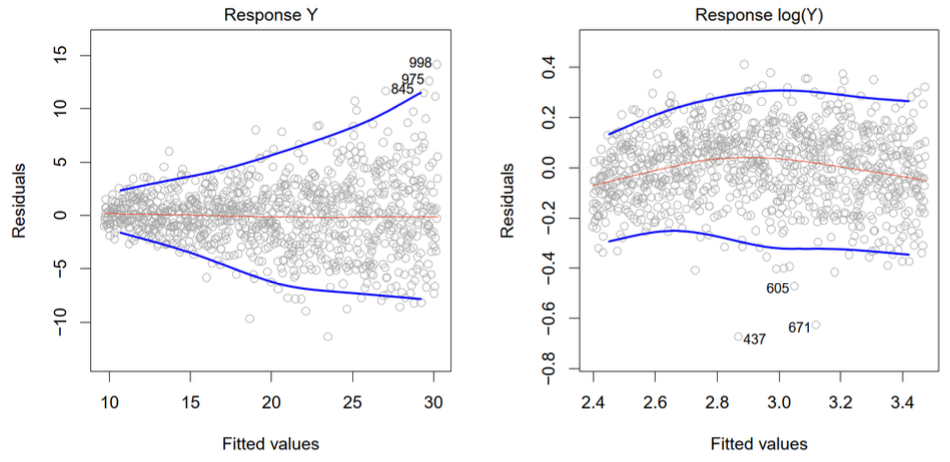
Heteroscedasticity (Non-constant Error Variance) Detection

Diagnostic Methods

Check scatter plot of residuals vs. fitted values (attachment page 25):

• Ideally, all residuals should have roughly the same variability

• Increasing (or decreasing) residual variability with fitted values indicates heteroscedasticity

• Since the sign of residuals is less important for detecting heteroscedasticity, often use scatter plots of $|e_i|$ or $e_i^2$ vs. $\hat{y_i}$

Effects of Heteroscedasticity

• Parameter estimates remain unbiased, but standard error estimates are biased

• t-tests and F-tests become invalid

• Confidence intervals and prediction intervals are inaccurate

Model Diagnostics: Error Term Tests

Dependence of Error Terms

In time series or spatial data, check scatter plots of residuals $e_i$ against time or geographical location:

• Purpose: Detect if there is correlation between adjacent residuals in the sequence

• Method: Plot $e_i$ against time or spatial location

• Ideal situation: Residuals should be randomly distributed, no specific pattern

Non-normality of Error Term

Three methods to test the normality of residuals $e_i$:

1. Distribution Plots

   • Histogram: Observe if the distribution shape is close to a bell curve
   • Box plot: Detect symmetry and outliers
   • Stem-and-leaf plot: Detailed display of data distribution characteristics

2. Cumulative Distribution Function Comparison

   • Estimate the sample cumulative distribution function
   • Compare with the theoretical normal cumulative distribution function
   • Large deviations indicate non-normality

3. Q-Q Plot (Quantile-Quantile Plot)

   • Principle: Compare sample quantiles with theoretical normal distribution quantiles
   • Judgment Criterion:
     • Points approximately on a straight line → Support normality assumption
     • Points significantly deviate from the line → Error terms are non-normal
   • Advantage: Sensitive to deviations from normality, good visualization effect

The core of model diagnostics is to verify whether the basic assumptions of linear regression hold, especially the i.i.d. and normality assumptions of the error terms $\epsilon_i$. These diagnostic tools help identify model defects and provide direction for model improvement.

Outlying Observations

Definition

• Outlier: An observation significantly separated from the majority of the data

• Classification:

  • Outlying Y observation (outlier): $y_i$ is far from the model predicted value
  • Outlying X observation (high leverage point): Observation with unusual X values

Detection Methods for Outlying Y Observations

Types of Residuals and Their Definitions

1. Ordinary Residuals and Semi-studentized Residuals

• Ordinary residual: $e_i = y_i - \hat{y}_i$

• Semi-studentized residual: $e_i^* = \frac{e_i}{\sqrt{MSE}}$

2. Studentized Residuals

• Definition: $r_i = \frac{e_i}{s(e_i)} = \frac{e_i}{\sqrt{MSE(1-h_{ii})}}$

• Characteristic: Accounts for differences in residual variability

3. Deleted Residual

• Definition: $d_i = y_i - \hat{y}_{i(-i)}$

  • $\hat{y}_{i(-i)}$: Model predicted value fitted without the i-th observation

• Property: $d_i = \frac{e_i}{1-h_{ii}}$

• Meaning: Simulates prediction error for a new observation

4. Studentized Deleted Residual

• Definition: $t_i = \frac{d_i}{s(d_i)} = \frac{e_i}{\sqrt{MSE_{(-i)}(1-h_{ii})}}$

• Distribution: $t_i \sim t_{n-p-2}$

• Calculation formula: $t_i = e_i \left[ \frac{n-p-2}{SSE(1-h_{ii}) - e_i^2} \right]^{1/2}$

Formal Test Methods

• Test statistic: Compare $|t_i|$ with $t(1-\frac{\alpha}{2n}, n-p-2)$

• Bonferroni correction: Adjust significance level to account for multiple testing

Detection of Outlying X Observations

Leverage

• Definition: Diagonal elements $h_{ii}$ of the hat matrix $H = X(X^TX)^{-1}X^T$

• Properties:

  • $0 \leq h_{ii} \leq 1$
  • $\sum_{i=1}^n h_{ii} = tr(H) = p+1$

• Meaning: Measures the distance of $x_i$ from the center of all X values

• Judgment criterion: $h_{ii} > \frac{2(p+1)}{n}$ indicates an outlying X observation

Outlier detection is an important part of model diagnostics. Outliers (Y anomalies) may be caused by measurement errors, while high leverage points (X anomalies) may have excessive influence on regression results. Through different residual definitions and leverage analysis, these outliers can be systematically identified and handled, improving model robustness.

Multicollinearity

Definition and Examples

• Multicollinearity: High correlation exists among predictor variables

• Ideal situation: Predictor variables are independent of each other (“independent variables” in statistics)

• Examples:

  • $Y \sim X_1(\text{weight}) + X_2(BMI) + \text{others}$
  • $Y \sim X_1(\text{credit rating}) + X_2(\text{credit limit}) + \text{others}$

Effects of Multicollinearity

• Variance of regression coefficient estimates becomes very large

• After deleting one variable, regression coefficients may change sign

• Marginal significance of predictor variables highly depends on other predictor variables included in the model

• Significance of predictor variables may be masked by correlated variables in the model

Variance Inflation Factor (VIF)

• Definition: $(\text{VIF})_j = (1 - R_j^2)^{-1}$

  • Where $R_j^2$ is the coefficient of determination obtained by regressing the j-th variable on the other $p-1$ variables in the model

• Judgment criterion:

  • Maximum VIF > 10 → Multicollinearity is considered to have an undue influence on least squares estimates
  • Average of all VIFs much greater than 1 → Indicates serious multicollinearity

Variable Transformation

Purpose

• Linearize nonlinear regression functions

• Stabilize error variance

• Normalize error terms

Box-Cox Transformation

• Transformation form: Use $y^\lambda$ ($\lambda \geq 0$) as the response variable, where $y^0$ is defined as $\ln(Y)$

• Choose optimal $\lambda$: Based on maximizing the likelihood function

  $$L(\lambda; \beta_0, \beta_1, \sigma^2) = \frac{1}{(2\pi\sigma)^{n/2}} \exp\left(-\frac{1}{2\sigma^2} \sum_{i=1}^n \left(y_i^{(\lambda)} - \beta_0 - \beta_1^T \mathbf{x}_i\right)^2\right)$$

Bias-Variance Tradeoff

Mean Squared Error (MSE) Decomposition

• Let $f_0(\mathbf{x})$ be the true regression function at $\mathbf{x}$, then the mean squared error of the estimator $\hat{f}(\mathbf{x})$ is:

  $$MSE(\hat{f}(\mathbf{x})) = E\left[ \left( \hat{f}(\mathbf{x}) - f_0(\mathbf{x}) \right)^2 \right]$$

• Decomposed as:

  $$MSE(\hat{f}(\mathbf{x})) = \text{var}(\hat{f}(\mathbf{x})) + \left[ E(\hat{f}(\mathbf{x})) - f_0(\mathbf{x}) \right]^2$$

  • First term: Variance (fluctuation of the estimator)
  • Second term: Squared bias (systematic error of the estimator)

Tradeoff Relationship and Regularization

• Gauss-Markov theorem: If the linear model is correct, the least squares estimator $\hat{f}$ is unbiased and has the smallest variance among all linear unbiased estimators of $y$

• Advantage of biased estimators: There may exist biased estimators with smaller MSE

• Regularization methods: Reduce variance through regularization, worthwhile if the increase in bias is small

  • Subset selection (forward, backward, all subsets)
  • Ridge Regression
  • Lasso regression

• Reality: Models are almost never completely correct, there is model bias between the “best” linear model and the true regression function

Multicollinearity seriously affects the interpretation and stability of regression coefficients and needs to be detected by indicators like VIF. Variable transformation is an effective means to improve model assumptions. The bias-variance tradeoff is the core issue in model selection; regularization methods may achieve smaller prediction errors by introducing bias to reduce variance.

Qualitative Predictors

Basic Model Setup

Consider a quantitative predictor variable $X_1$ and a qualitative predictor with two levels $M_1$ and $M_2$:

Dummy Variable Coding

• Definition: $X_2 = \begin{cases} 1 & \text{if level } M_1 \\ 0 & \text{if level } M_2 \end{cases}$

• Regression model: $E(Y|X) = \beta_0 + \beta_1X_1 + \beta_2X_2$

Model Interpretation

• For level $M_1$: $E(Y|X) = \beta_0 + \beta_1X_1 + \beta_2$

• For level $M_2$: $E(Y|X) = \beta_0 + \beta_1X_1$

• Geometric meaning: Parallel lines with different intercepts but same slope

• Parameter meaning: $\beta_2 = E(Y|X_2=1) - E(Y|X_2=0) = E(Y|M_1) - E(Y|M_2)$

  • $\beta_2$ represents the difference in average response between the two levels

Interaction Effects

Model with Interaction Term

• Model form: $E(Y|X) = \beta_0 + \beta_1X_1 + \beta_2X_2 + \beta_3X_1X_2$

• Model interpretation:

  • For level $M_1$: $E(Y|X) = (\beta_0 + \beta_2) + (\beta_1 + \beta_3)X_1$
  • For level $M_2$: $E(Y|X) = \beta_0 + \beta_1X_1$

Meaning of Interaction Effects

• Geometric meaning: Non-parallel lines with different intercepts and slopes

• Parameter interpretation:

  • $\beta_2$: Difference in intercepts between the two levels at $X_1=0$
  • $\beta_3$: Difference in slopes between the two levels

• Interaction term: $X_1X_2$ allows the slope to vary with the level of the qualitative variable

Extended Explanation

Multiple Qualitative Predictors

• Can include multiple qualitative predictors

• Each qualitative variable needs separate coding

Multi-level Qualitative Variables

For a qualitative variable with 5 levels, coding methods:

Method 1: Ordinal Coding (Not Recommended)

• Directly code as 1, 2, 3, 4, 5

• Problem: Implies ordinal relationship, may not reflect reality

Method 2: Dummy Variable Coding (Recommended)

• Define 4 dummy variables $X_1, X_2, X_3, X_4$

• $X_j = 1$ if level $j$, otherwise 0 ($j=1,2,3,4$)

• Baseline level: The 5th level serves as the reference baseline

Method 3: Effect Coding

• Define $X_1, X_2, X_3, X_4$

• $X_j = 1$ if level $j$, $X_j = -1$ if level 5, otherwise 0

• Characteristic: Parameters represent deviations from the overall mean

Qualitative predictors are introduced into the regression model through dummy variable coding. Interaction effects allow different groups to have different slopes. Multi-level qualitative variables require careful coding to avoid spurious ordinal relationships; dummy variable coding is the most commonly used method. Correct coding is essential for model interpretation and statistical inference.