SDSC6007 Course 1

#sdsc6007

English / 中文

Introduction

The Discrete-Time Dynamic System

The system has the form

$$x_{k + 1} = f_{k} (x_k, u_k, w_k ), k = 0, 1, . . . , N − 1,$$

where

• $k$ : index of discrete time

• $N$ : the horizon or number of times control is applied

• $x_k$ : the state of the system, from the set of states Sk

• $u_k$ : the control/decision variable/action to be selected from the set Uk (xk ) at time k

• $w_k$ : a random parameter (also called disturbance)

• $f_k$ : a function that describes how the state is updated

Assumption
$w_k$ ’s are independent. The probability distribution may depend on $x_k$ and $u_k$ .

The Cost Function

The (expected) cost has the form

$$\mathbb{E} \left[ g_N (x_N ) + \sum^{N−1}_{k=0}{g_k (x_k, u_k, w_k )} \right]$$

where

• $g_k(x_k, u_k, w_k)$ : the cost incurred at time $k$.

• $g_N(x_N)$ : the terminal cost incurred at the end of process.

Note
Because of $w_k$ , the cost is a random variable and so we are optimizing over the expectation.

A Deterministic Scheduling Problem

Example
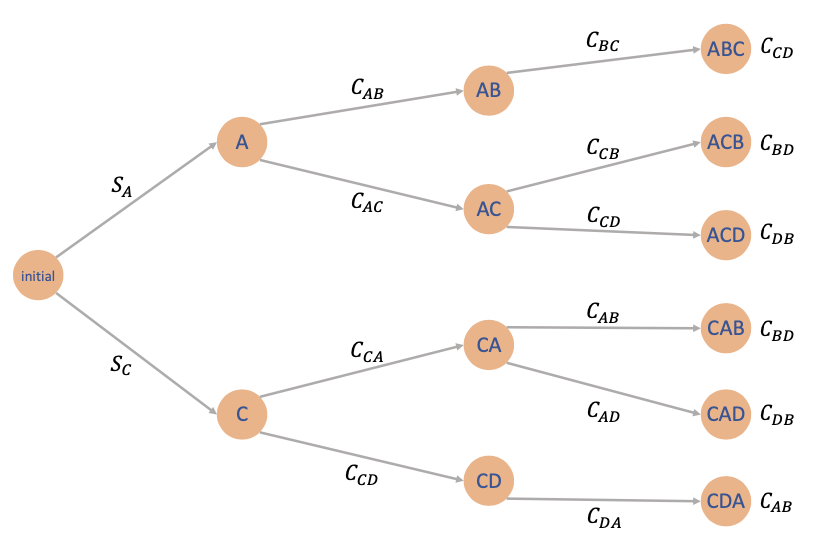
Prof wants to produce luxury headphones that perform better than the bear-pods 3 that he is currently using. To do so, four operations must be performed on a certain machine, and they are denoted by A, B, C, D. Assuming that

1. operation B can only be performed after operation A

2. operation D can only be performed after operation C

Denote

• setup cost Cmn for passing any operation m to n

• initial startup cost SA or SC (can only start with operation A or C)

Solution

• We need to make three decisions (the last is determined by the first three)

• This problem is deterministic (no wk )

• This problem has finite number of states

• Deterministic problems with finite number of states => transition graph

Discrete-State and Finite-State Problems

To capture the transition between states, it is often convenient to define the transition probabilities

$$p_{ij}(u,k) = \mathbb{P}(x_{k+1} = j | x_k = i, u_k = u)$$

In the dynamic system, it means that $x_{k+1} = w_k$, where $w_k$ follows a probabilitydistribution which has probabilities $p_{ij}(u,k)$'s.

Example

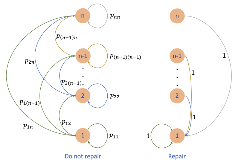
Consider a problem of N time periods that a machine can be in any one of n states. We denote $g(i)$ as the operating cost per period when the machine is in state i. Assume that

$$g(1) ≤ g(2) ≤ ··· ≤ g(n)$$

That is, a machine in state i works more efficiently than a machine that is in state i + 1. During a period of time, the state of the machine can become worse or stay the same with probability

$$p_{ij} =\mathbb{P}(\text{next state will be } j | \text{current state is } i ) \text{ and } p_{ij} =0,\text{if} j < i.$$

At the start of each period, we can choose

• let the machine operate one more period

• repair the machine and bring it to state 1 (and it will stay there for 1 period) at a cost R

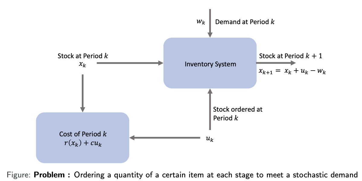
Inventory Control Problem

Ordering a quantity of a certain item at each stage to meet a stochastic demand

• $x_k$: stock available at the beginning of the kth period

• $u_k$: stock ordered and delivered at the beginning of the kth period

• $w_k$: demand during the kth period with given probability distribution

• $r(·)$: penalty/cost for either positive or negative stock

• $c$: cost per unit ordered

Expample: Inventory Control

Suppose $(u_0^{\star}, u_1^\star, \ldots, u_{N-1}^\star)$ is the optimal solution of

$$\min \mathbb{E} \left[ R(x_N) + \sum_{k=0}^{N-1} \left( r(x_k + u_k - w_k) + c \cdot u_k \right) \right]$$

What if:$w_1 = w_2 = \cdots = w_{N-1} = 0$? (recall wi’s are the demands.)

We can do better if we can adjust our decisions to different situations!

Open-Loop and Closed-Loop Control

Open-loop Control

At initial time $k=0$, given initial state $x_0$, find optimal control sequence $(u_0^\star, u_1^\star, \ldots, u_{N-1}^\star)$ minimizing expected total cost:

• Key feature: Subsequent state information is NOT used to adjust control decisions

Closed-loop Control

At each time $k$, make decisions based on current state information $x_k$ (e.g. ordering decision at time $k$):

• Core objective: Find state feedback strategy $\mu_k(\cdot)$ mapping state $x_k$ to control $u_k$

• Decision characteristics:

• Re-optimization at each decision point $k$

• Control rule designed for every possible state value $x_k$

• Computational properties:

• Higher computational cost (requires real-time state mapping)

• Same performance as open-loop when no uncertainty exists

Closed-loop Control

Core Concepts

• Control Law Definition
  Let $\mu_k(\cdot)$ be a function mapping state $x_k$ to control $u_k$:

$$u_k = \mu_k(x_k)$$

• Control Policy
  Define a policy $\pi$ as a sequence of control laws:

$$\pi = {\mu_0, \mu_1, \ldots, \mu_{N-1}}$$

• Policy Cost Function
  Given initial state $x_0$, the expected cost of policy $\pi$ is:

$$J_{\pi}(x_0) = \mathbb{E} \left[ g_N (x_N) + \sum_{k=0}^{N-1} g_k \big( x_k, \mu_k(x_k), w_k \big) \right]$$

Admissible Policy

A policy $\pi = \{\mu_0, \ldots, \mu_{N-1}\}$ is called admissible if and only if:

$$\mu_k(x_k) \in U_k(x_k), \quad \forall x_k \in S_k, \ \forall k = 0,1,\ldots,N-1$$

Meaning at each time $k$ and for every possible state $x_k$, the control $u_k$ must belong to the allowable control set $U_k(x_k)$.

Summary

Definition

Consider a function $J^*$ defined as:

$$J^*(x_0) = \min_{\pi \in \Pi} J^{\pi}(x_0), \quad \forall x_0 \in S_0$$

where:

• $\Pi$: Set of all admissible policies

• $J^{\pi}(x_0)$: Expected cost of policy $\pi$ starting from initial state $x_0$

We call $J^*$ the optimal value function.

Key Properties

1. Global Optimality
   $J^*$ gives the minimum possible expected cost from any initial state $x_0$

2. Policy Independence
   Represents theoretical performance limit, independent of specific policies

3. Benchmarking Role
   Any admissible policy $\pi$ satisfies:

$$J^{\pi}(x_0) \geq J^*(x_0), \quad \forall x_0 \in S_0$$

Computational Significance

• Core Objective of DP: Compute $J^*$ exactly via backward induction

• Control Engineering Application: Measure gap between actual policies and theoretical optimum

The Dynamic Programming Algorithm

Principle of Optimality

Theorem Statement

Let $\pi^* = \{\mu_0^*, \mu_1^*, \ldots, \mu_{N-1}^*\}$ be an optimal policy for the basic problem. Suppose when using $\pi^*$, the system reaches state $x_i$ at time $i$ with positive probability. Consider the subproblem starting from $(x_i, i)$:

$$\min \mathbb{E} \left[ g_N(x_N) + \sum_{k=i}^{N-1} g_k \big( x_k, \mu_k(x_k), w_k \big) \right]$$

Then the truncated policy $\{\mu_i^*, \mu_{i+1}^*, \ldots, \mu_{N-1}^*\}$ is optimal for this subproblem.

Core Implications

• Piecemeal Construction: Optimal policy can be constructed in piecemeal fashion

• Tail First: First solve the “tail subproblem” (starting from final stage)

• Sequential Extension: Extend sequentially to the original problem

1. Heritability of Optimality
   Any tail portion of a globally optimal policy remains optimal for its starting state

2. Time Consistency
   Optimal decisions account for both immediate cost and optimal future state evolution

3. Foundation for Backward Induction
   This principle validates the dynamic programming backward solution approach.

DP Algorithm - Inventory Control Example

Example

Tail Subproblem Solving Process

Core idea: Backward solution from final stage to initial stage

1. Length-1 Tail Subproblem (at $k = N-1$)

   • Decision Objective: Minimize current cost + terminal cost expectation

     $$\text{minimize} \quad c \cdot u_{N-1} + \mathbb{E}_{w_{N-1}} \left[ R(x_N) \right]$$

     • $c \cdot u_{N-1}$: Current ordering cost
     • $\mathbb{E}_{w_{N-1}} \left[ R(x_N) \right]$: Expected terminal inventory cost

   • State Transition: $x_N = x_{N-1} + u_{N-1} - w_{N-1}$

     $$\Rightarrow \text{minimize} \quad c \cdot u_{N-1} + \mathbb{E}_{w_{N-1}} \left[ R(x_{N-1} + u_{N-1} - w_{N-1}) \right]$$

   • Value Function Calculation:

     $$J_{N-1}(x_{N-1}) = r(x_{N-1}) + \min_{u_{N-1} \geq 0} \left\{ c \cdot u_{N-1} + \mathbb{E}_{w_{N-1}} \left[ R(x_{N-1} + u_{N-1} - w_{N-1}) \right] \right\}$$

     • $r(x_{N-1})$: Current holding/shortage cost
     • Compute for all $x_{N-1} \in S_{N-1}$

2. Length-2 Tail Subproblem (at $k = N-2$)

   • Decision Objective: Minimize current cost + expected future cost

     $$\text{minimize} \quad r(x_{N-2}) + c \cdot u_{N-2} + \mathbb{E}_{w_{N-2}} \left[ J_{N-1}(x_{N-1}) \right]$$

   • State Transition: $x_{N-1} = x_{N-2} + u_{N-2} - w_{N-2}$

     $$\Rightarrow \text{minimize} \quad r(x_{N-2}) + c \cdot u_{N-2} + \mathbb{E}_{w_{N-2}} \left[ J_{N-1}(x_{N-2} + u_{N-2} - w_{N-2}) \right]$$

   • Value Function Calculation:

     $$J_{N-2}(x_{N-2}) = r(x_{N-2}) + \min_{u_{N-2} \geq 0} \left\{ c \cdot u_{N-2} + \mathbb{E}_{w_{N-2}} \left[ J_{N-1}(x_{N-2} + u_{N-2} - w_{N-2}) \right] \right\}$$

3. General Recursion (Length $N-k$ Tail Subproblem)

   $$J_k(x_k) = r(x_k) + \min_{u_k \geq 0} \left\{ c \cdot u_k + \mathbb{E}_{w_k} \left[ J_{k+1}(x_k + u_k - w_k) \right] \right\}$$

   • $r(x_k)$: Inventory cost at $k$
   • $c \cdot u_k$: Ordering cost at $k$
   • $\mathbb{E}_{w_k} \left[ J_{k+1}(\cdot) \right]$: Expected optimal future cost

Final Goal: Solve original problem via length-$N$ tail subproblem at $k=0$

The Dynamic Programming Algorithm

For every initial state $x_0$, the optimal cost $J^*(x_0)$ equals $J_0(x_0)$ computed by:

Boundary Condition:

$$J_N(x_N) = g_N(x_N)$$

Recursive Relation:

$$J_k(x_k) = \min_{u_k \in U_k(x_k)} \mathbb{E}_{w_k} \left[ g_k(x_k,u_k,w_k) + J_{k+1}\big(f_k(x_k,u_k,w_k)\big) \right] \quad (\star)$$

The expectation $\mathbb{E}_{w_k}$ is over $w_k$’s probability distribution (dependent on $x_k$ and $u_k$). If $u_k^\star = \mu_k^\star(x_k)$ minimizes the RHS of $(\star)$, then $\pi^\star = \{\mu_0^\star, \ldots, \mu_{N-1}^\star\}$ is optimal.

Key Definitions

• $J_k(x_k)$: Cost-to-go at state $x_k$ and time $k$

• $J_k$: Cost-to-go function at time $k$

Algorithm Proof (Informal)

Setup

1. Define subpolicy $\pi_k = \{\mu_k, \mu_{k+1}, \ldots, \mu_{N-1}\}$

2. Let $J_k^\star(x_k)$ be optimal cost for $(N-k)$-stage starting at $(x_k, k)$:

$$J_k^\star(x_k) = \min_{\pi_k} \mathbb{E}_{w_k,\ldots,w_{N-1}} \left[ g_N(x_N) + \sum_{i=k}^{N-1} g_i\big(x_i, \mu_i(x_i), w_i\big) \right]$$

3. Boundary conditions:

   • At $k=0$: $J_0^\star$ solves original problem
   • At $k=N$: $J_N^\star = g_N(x_N)$

Inductive Proof

Goal: Prove $J_k^\star = J_k$ (DP algorithm value)

1. Base Case: Holds at $k=N$ ($J_N^\star = g_N(x_N) = J_N$)

2. Induction Hypothesis: Assume $\forall x_{k+1} \in S_{k+1}$, $J_{k+1}^\star(x_{k+1}) = J_{k+1}(x_{k+1})$

3. Derivation:

$$\begin{align*} J_k^\star(x_k) &= \min_{(\mu_k, \pi_{k+1})} \mathbb{E}_{w_k,\ldots,w_{N-1}} \left[ g_N(x_N) + \sum_{i=k}^{N-1} g_i\big(x_i, \mu_i(x_i), w_i\big) \right] \\ &= \min_{(\mu_k, \pi_{k+1})} \mathbb{E} \left[ g_k(x_k, \mu_k(x_k), w_k) + g_N(x_N) + \sum_{i=k+1}^{N-1} g_i(\cdots) \right] \\ &= \min_{\mu_k} \mathbb{E}_{w_k} \left[ g_k(x_k, \mu_k(x_k), w_k) + \min_{\pi_{k+1}} \mathbb{E}_{w_{k+1},\ldots,w_{N-1}} \left[ g_N(x_N) + \sum_{i=k+1}^{N-1} g_i(\cdots) \right] \right] \\ &\quad \text{(Principle of Optimality)} \\ &= \min_{\mu_k} \mathbb{E}_{w_k} \left[ g_k(x_k, \mu_k(x_k), w_k) + J_{k+1}^\star\big(f_k(x_k, \mu_k(x_k), w_k)\big) \right] \\ &= \min_{\mu_k} \mathbb{E}_{w_k} \left[ g_k(x_k, \mu_k(x_k), w_k) + J_{k+1}\big(f_k(x_k, \mu_k(x_k), w_k)\big) \right] \\ &\quad \text{(by Induction Hypothesis)} \\ &= \min_{u_k} \mathbb{E}_{w_k} \left[ g_k(x_k, u_k, w_k) + J_{k+1}\big(f_k(x_k, u_k, w_k)\big) \right] \\ &= J_k(x_k) \end{align*}$$

DP Algorithm - Baking Example

Problem Description

Dr. Yang bakes a cake using two ovens with dynamics and cost:

• State equation: $x_{k+1} = (1-a) \cdot x_k + a \cdot u_k, \quad k=0,1$

• Cost function: $r \cdot (x_2 - T)^2 + u_0^2 + u_1^2$

• Parameters:

  • $x_k$: Cake temperature at exit of oven $k$
  • $u_k$: Set temperature of oven $k$
  • $a \in (0,1)$: Heat transfer coefficient
  • $T$: Target temperature
  • $r > 0$: Penalty for terminal temperature deviation

DP Solution Process

1. Terminal Time ($k=2$)

$$J_2(x_2) = r \cdot (x_2 - T)^2$$

2. Time $k=1$

$$\begin{align*} J_1(x_1) &= \min_{u_1} \left[ u_1^2 + J_2(x_2) \right] \\ &= \min_{u_1} \left[ u_1^2 + r \cdot \big((1-a)x_1 + a u_1 - T\big)^2 \right] \end{align*}$$

Optimization:

• Set derivative w.r.t $u_1$ to zero:

  $$0 = 2u_1 + 2ra \big((1-a)x_1 + a u_1 - T\big)$$

• Optimal control:

  $$u_1^* = \frac{ra \big(T - (1-a)x_1\big)}{1 + ra^2}$$

• Value function:

  $$J_1(x_1) = \frac{r \big((1-a)x_1 - T\big)^2}{1 + ra^2}$$

3. Initial Time ($k=0$)

$$\begin{align*} J_0(x_0) &= \min_{u_0} \left[ u_0^2 + J_1(x_1) \right] \\ &= \min_{u_0} \left[ u_0^2 + \frac{r \big((1-a)^2 x_0 + (1-a)a u_0 - T\big)^2}{1 + ra^2} \right] \end{align*}$$

Optimization:

• Optimal control:

  $$u_0^* = \frac{r(1-a)a \big(T - (1-a)^2 x_0\big)}{1 + ra^2 \big(1 + (1-a)^2\big)}$$

• Value function:

  $$J_0(x_0) = \frac{r \big((1-a)^2 x_0 - T\big)^2}{1 + ra^2 \big(1 + (1-a)^2\big)}$$

Key Insight:
This LQ problem admits analytical solution, but most DP problems require numerical methods

DP Algorithm - Inventory Control Example

Problem Setup

• Demand Handling: Unmet demand is lost

• State Transition: $x_{k+1} = \max\{0, x_k + u_k - w_k\}$

• Control Constraint: $x_k + u_k \leq 2$

• Cost Structure:

  • Ordering cost: $u_k$ (unit cost=1)
  • Holding cost: $(x_k + u_k - w_k)^2$
  • Terminal cost: $g_N(x_N) = 0$

• Demand Distribution:
  $P(w_k=0)=0.1,\ P(w_k=1)=0.7,\ P(w_k=2)=0.2$

• Initial State: $x_0=0,\ N=3$

Backward Solution Process

需要注意，由于此时 $u_k$ 为随机分布，因此计算得到的 $J_k$ 为数学期望。
It should be noticed that, as $u_k$ is random distribution in this case, thus $J_k$ is mathematical expectation.

1. Terminal Time ($k=3$)

$$J_3(x_3) = 0 \quad (\forall x_3)$$

2. Time $k=2$ (Penultimate Stage)

State Space: $x_2 \in \{0,1,2\}$

• $x_2=0$:

  $$\begin{align*} J_2(0) &= \min_{u_2 \in \{0,1,2\}} \mathbb{E}_{w_2} \left[ u_2 + (0 + u_2 - w_2)^2 \right] \\ &= \min \begin{cases} u_2=0: & 0 + 0.1(0)^2 + 0.7(-1)^2 + 0.2(-2)^2 = 1.5 \\ u_2=1: & 1 + 0.1(1)^2 + 0.7(0)^2 + 0.2(-1)^2 = 1.3 \\ u_2=2: & 2 + 0.1(4) + 0.7(1) + 0.2(0) = 3.1 \end{cases} \\ &= 1.3 \quad (u_2^*=1) \end{align*}$$

• $x_2=1$:

  $$\begin{align*} J_2(1) &= \min_{u_2 \in \{0,1\}} \mathbb{E}_{w_2} \left[ u_2 + (1 + u_2 - w_2)^2 \right] \\ &= \min \begin{cases} u_2=0: & 0 + 0.1(1)^2 + 0.7(0)^2 + 0.2(-1)^2 = 0.3 \\ u_2=1: & 1 + 0.1(4) + 0.7(1) + 0.2(0) = 2.1 \end{cases} \\ &= 0.3 \quad (u_2^*=0) \end{align*}$$

• $x_2=2$:

  $$\begin{align*} J_2(2) &= \min_{u_2 \in \{0\}} \mathbb{E}_{w_2} \left[ u_2 + (2 + u_2 - w_2)^2 \right] \\ &= 0 + 0.1(4) + 0.7(1) + 0.2(0) = 1.1 \quad (u_2^*=0) \end{align*}$$

Value Function Summary:

$x_2$	$J_2(x_2)$	$\mu_2^*(x_2)$
0	1.3	1
1	0.3	0
2	1.1	0

3. Continue to $k=1,0$

Similar computation for $J_1(x_1)$ and $J_0(x_0)$, considering state transition:

$$x_{k+1} = \max\{0, x_k + u_k - w_k\}$$

Computational Complexity

• State Space: $|S_k| = 3$ (this example)

• Control Space: $|U_k| \leq 3$ (this example)

• Time Complexity: $O(N \cdot |S| \cdot |U| \cdot |W|)$

• Practical Challenge: State space grows exponentially with dimensions (curse of dimensionality)

DP Algorithm - Finite-State Systems

System Description

Consider finite-state systems with:

• Transition probability: $p_{ij}(u) = \mathbb{P}(x_{k+1} = j \mid x_k = i, u_k = u)$

• Dynamics: $x_{k+1} = w_k$ where $w_k$ follows distribution defined by $p_{ij}(u)$

Key Assumptions

1. Stationarity:

   • Transition probabilities $p_{ij}(u)$ time-invariant
   • Control constraint sets $U_k(i) = U(i)$ constant

2. Cost Structure:

   • Stage cost $g(i,u)$ independent of disturbance $w_k$

DP Algorithm

Recursive Formula:

$$J_k(i) = \min_{u \in U(i)} \left[ g(i,u) + \mathbb{E} \left[ J_{k+1}(w_k) \right] \right]$$

Explicit Form:

$$J_k(i) = \min_{u \in U(i)} \left[ g(i,u) + \sum_{j} p_{ij}(u) J_{k+1}(j) \right]$$

Computational Properties

Property	Description
State Space	Finite ($i \in \{1,2,\dots,n\}$)
Action Space	Finite ($u \in U(i)$)
Complexity	$O(N \cdot n^2 \cdot
Advantage	Avoids curse of dimensionality

Applications: Markov Decision Processes (MDP), queueing systems, network routing

State Augmentation and System Reformulation

1. Handling Time Lags

Problem: When state transition depends on historical states (e.g., $x_{k+1} = f_k(x_k, x_{k-1}, u_k, u_{k-1}, w_k)$)

Solution: State Augmentation
Define new state vector:

$$\tilde{x}_k = \begin{bmatrix} x_k \\ y_k \\ s_k \end{bmatrix} = \begin{bmatrix} x_k \\ x_{k-1} \\ u_{k-1} \end{bmatrix}$$

New state transition:

$$\tilde{x}_{k+1} = \begin{bmatrix} x_{k+1} \\ y_{k+1} \\ s_{k+1} \end{bmatrix} = \begin{bmatrix} f_k(x_k, y_k, u_k, s_k, w_k) \\ x_k \\ u_k \end{bmatrix} = \tilde{f}_k(\tilde{x}_k, u_k, w_k)$$

Key: Embed historical state $x_{k-1}$ and control $u_{k-1}$ into current state

---

2. Handling Correlated Disturbances

Problem: Correlated disturbances (e.g., $w_k = \lambda w_{k-1} + \xi_k$)

Solution: State Augmentation
Define new state vector:

$$\tilde{x}_k = \begin{bmatrix} x_k \\ y_k \end{bmatrix} \quad \text{where} \quad y_k = w_{k-1}$$

New state transition:

$$\tilde{x}_{k+1} = \begin{bmatrix} x_{k+1} \\ y_{k+1} \end{bmatrix} = \begin{bmatrix} f_k(x_k, u_k, \lambda y_k + \xi_k) \\ \lambda y_k + \xi_k \end{bmatrix} = \tilde{f}_k(\tilde{x}_k, u_k, \xi_k)$$

Generalized: For $w_k = C_k y_{k+1}$, $y_{k+1} = A_k y_k + \xi_k$:

$$\tilde{x}_{k+1} = \begin{bmatrix} f_k(x_k, u_k, C_k(A_k y_k + \xi_k)) \\ A_k y_k + \xi_k \end{bmatrix}$$

---

3. Incorporating Forecast Information

Problem: Disturbance distribution known before decision (e.g., weather affecting demand)

Modeling:

• $w_k \sim Q_i$ ($i \in \{1,\dots,m\}$)

• $i$ known before deciding $u_k$

• Forecast process: $y_{k+1} = \xi_k$ ($\xi_k$ independent, $P(\xi_k=i)=p_i$)

Augmented state:

$$\tilde{x}_k = \begin{bmatrix} x_k \\ y_k \end{bmatrix}$$

where $y_k$ encodes next-period disturbance distribution

State transition:

$$\tilde{x}_{k+1} = \begin{bmatrix} x_{k+1} \\ y_{k+1} \end{bmatrix} = \begin{bmatrix} f_k(x_k, u_k, w_k) \\ \xi_k \end{bmatrix}$$

Decision advantage: $u_k$ can leverage $y_k$ (future disturbance distribution)