SDSC6007 Course 2

#sdsc6007

English / 中文

Shortest Path Problems (SPP)

Problem Definition

Given node set $\{1,2,\dots,N,t\}$ ($t$=destination),

• $a_{ij}$: Cost from node $i$ to $j$ ($a_{ij} = \infty$ if no direct path)

• Key assumption: All cycles have non-negative cost ($\forall \text{ cycles } i \to j_1 \to \cdots \to j_k \to i,\ \text{total cost} \geq 0$)

• Goal: Find min-cost path from any $i$ to $t$

Significance of Non-negative Cycle Assumption

Core implication: Guarantees existence of optimal solution with finite path length

1. Prevents infinite cost reduction:

   $$\text{If } \exists \text{ negative cycle } \sum_{\text{cycle}} a_{ij} < 0 \Rightarrow \text{total cost can be arbitrarily reduced}$$

   Example: Repeated traversal of negative-cost cycle drives cost to $-\infty$

2. Self-loop constraint:

   $$a_{ii} \geq 0 \quad (\text{if self-transitions allowed})$$

3. Path length bound:

   $$\text{Optimal path contains at most } N \text{ moves}$$

   • Can enforce exactly $N$ moves by setting $a_{ii} = 0$ (allowing self-loops)

Dynamic Programming Formulation

Define value function:

$$J_k(i) = \text{Min cost from } i \text{ to } t \text{ in exactly } k \text{ steps}$$

Recursion:

$$J_k(i) = \min_{j} \left[ a_{ij} + J_{k-1}(j) \right]$$

Boundary conditions:

$$J_0(t) = 0, \quad J_0(i) = \infty \ (i \neq t)$$

​​Practical meaning of non-negative cycle assumption​​:

This assumption ensures the shortest path problem is well-posed with a finite optimal solution. Negative-cost cycles would cause algorithms to loop indefinitely without convergence.

In real-world applications (routing, network optimization), this condition is naturally satisfied when costs represent physical quantities like distance or latency.

Deterministic Dynamic Programming

Characteristics of Deterministic Systems

Key feature: No stochastic disturbance ($w_k$ absent or known constant)

1. Fully predictable state transition:

   $$x_{k+1} = f_k(x_k, u_k)$$

   • State trajectory can be exactly computed given $x_0$ and policy $\{\mu_0,\dots,\mu_{N-1}\}$

2. No advantage of closed-loop control:

   $$J^{\text{closed-loop}} = J^{\text{open-loop}}$$

   • Optimal open-loop sequence $(u_0^*,u_1^*,\dots,u_{N-1}^*)$ achieves same cost as closed-loop policy

Why no closed-loop advantage:

In deterministic systems, future states are entirely determined by current decisions. State feedback provides no new information, so closed-loop policies cannot improve upon precomputed open-loop sequences.

Finite-State System Modeling

State transition graph representation:

• Nodes: States $x_k \in \mathcal{S}_k$ (finite set)

• Directed edges: State transitions driven by control $u_k$

  $$x_k \xrightarrow{u_k} x_{k+1} = f_k(x_k, u_k)$$

• Edge cost: Stage cost $g_k(x_k, u_k)$

Key simplification:

For each state transition $x_k \to x_{k+1}$, keep only minimum-cost decision:

$$c_k(x_k, x_{k+1}) = \min_{\substack{u_k \in U_k(x_k) \\ f_k(x_k,u_k)=x_{k+1}}} g_k(x_k, u_k)$$

Dynamic Programming Equations

Value function recursion:

$$J_k(x_k) = \min_{x_{k+1}} \left[ c_k(x_k, x_{k+1}) + J_{k+1}(x_{k+1}) \right]$$

Boundary condition:

$$J_N(x_N) = g_N(x_N)$$

Computational implication: Transforms problem into multi-stage shortest path

Essence of finite-state systems:

Modeling as state transition graphs reduces the problem to finding minimum-cost paths. DP becomes a backward graph traversal algorithm in this context.

Equivalence: Deterministic Finite-State Systems & Shortest Path Problems

Deterministic System → SPP

Transformation:

1. Define nodes:

   • $s$: Initial state node (corresponds to $x_0$)
   • $t$: Terminal node (artificially added)

2. Edge costs:

   • Stage $k$ transition: $a_{ij}^k = \min_{u_k} g_k(i, u_k)$ (when $f_k(i,u_k)=j$)
     • $i$: Current state
     • $j$: Next state
     • $u_k$: Control decision
     • $g_k$: Stage cost function
   • Terminal cost: $a_{it}^N = g_N(i)$
     • $g_N$: Terminal cost function

3. Path cost:

   $$\text{Total cost} = \sum_{k=0}^{N-1} a_{x_k x_{k+1}}^k + a_{x_N t}^N$$

Core equivalence: Optimal cost $= J_0(s) =$ Shortest path length from $s$ to $t$

Backward DP Algorithm

Value function:

$$J_k(i) = \text{Min cost from state } i \text{ at stage } k \text{ to terminal } t$$

• $k$: Current stage

• $i$: Current state

Recursion:

$$\begin{aligned} J_N(i) &= a_{it}^N \quad \forall i \in S_N \\ & \quad \text{(Terminal cost: direct cost from state } i \text{ to } t\text{)} \\ J_k(i) &= \min_{j \in S_{k+1}} \left[ a_{ij}^k + J_{k+1}(j) \right] \quad k = N-1,\dots,0 \\ & \quad \text{(Minimize: transition cost } a_{ij}^k \text{ + optimal future cost } J_{k+1}(j)\text{)} \end{aligned}$$

Optimal solution: $J_0(s)$ gives shortest path length (min cost from initial state $s$ to terminal $t$)

SPP → Deterministic System

Transformation:

1. Fix number of stages $N$ (guaranteed by non-negative cycles)

2. Value function:

   $$J_k(i) = \text{Min cost from } i \text{ to } t \text{ in } N-k \text{ steps}$$

   • $N-k$: Remaining steps

3. Recursion:

   $$\begin{aligned} J_{N-1}(i) &= a_{it} \\ & \quad \text{(One-step transition cost)} \\ J_k(i) &= \min_{j=1,\dots,N} \left[ a_{ij} + J_{k+1}(j) \right] \quad k=0,\dots,N-2 \\ & \quad \text{(Minimize: current transition cost } a_{ij} \text{ + optimal future cost } J_{k+1}(j)\text{)} \end{aligned}$$

Key point: $J_0(i)$ gives shortest path cost from $i$ to $t$

Forward DP Algorithm (Special Property)

Only for deterministic SPP:

• Value function:

  $$\tilde{J}_k(j) = \text{Min cost from } s \text{ to } j \text{ (stage } k\text{)}$$

  • $k$: Current stage
  • $j$: Current state

• Recursion:

  $$\begin{aligned} \tilde{J}_1(j) &= a_{sj}^0 \quad \forall j \in S_1 \\ & \quad \text{(Cost from initial state } s \text{ to stage 1 state } j\text{)} \\ \tilde{J}_k(j) &= \min_{i \in S_{k-1}} \left[ a_{ij}^{N-k+1} + \tilde{ J}_{k-1}(i) \right] \quad k=2,\dots,N \\ & \quad \text{(Minimize: transition cost } a_{ij}^{N-k+1} \text{ + optimal past cost } \tilde{J}_{k-1}(i)\text{)} \\ \tilde{J}_0(t) &= \min_{i \in S_N} \left[ a_{it}^N + \tilde{J}_N(i) \right] \\ & \quad \text{(Terminal cost: from state } i \text{ to } t \text{ + optimal cost to } i\text{)} \end{aligned}$$

Comparison:
Backward DP computes “cost-to-go”, forward DP computes “cost-to-arrive”.
Equivalent in deterministic SPP due to path symmetry, but forward method inapplicable to stochastic problems.

Shortest Path Application: Critical Path Analysis

Problem Description

Application scenario: Activity scheduling optimization in project management

Core objectives:

1. Determine minimum project duration

2. Identify critical activities (delays cause project delay)

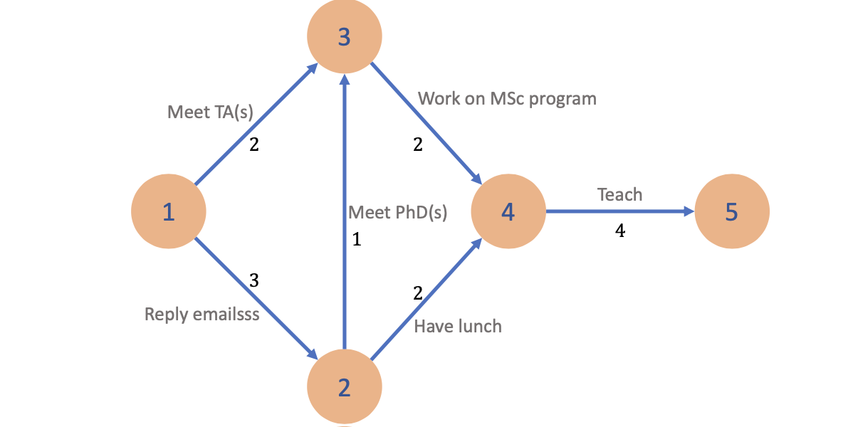
Case Study: Dr. Yang’s Schedule Optimization

Activity decomposition:

Activity	Description
Meeting with TAs	Must complete
Replying emails
Lunch
Meeting with PhD students
MSc program work
Teaching

Phase division:

• Nodes represent schedule phases ($N=5$)

• Edge $(i,j)$ represents activity with duration $t_{ij}>0$

• Node 1: Start of day (no incoming edges)

• Node 5: End of day (no outgoing edges)

Critical Path Algorithm

Variable	Symbol	Definition
Path Duration	$D_p$	Total duration of path $p$ Calculation: $D_p = \sum_{(i,j)\in p} t_{ij}$
Earliest Completion Time	$T_i$	Earliest completion time at node $i$ Calculation: $T_i = \max_{\text{all paths } p \text{ from 1 to } i} D_p$
Activity Duration	$t_{ji}$	Duration of activity $(j,i)$ (Edge weight from node $j$ to $i$)
Predecessor Set	$\text{Pred}(i)$	Set of direct predecessor nodes of $i$ (Nodes with edges pointing directly to $i$)
Critical Activity Condition	$T_i = T_j + t_{ji}$	Necessary and sufficient condition for activity $(j,i)$ to be critical (Activity has zero slack when this holds)
Slack Time	$\text{Slack}_{ji}$	Delay tolerance for non-critical activities Calculation: $\text{Slack}_{ji} = T_i - (T_j + t_{ji})$

Path duration calculation:

$$D_p = \sum_{(i,j)\in p} t_{ij} \quad \text{(total duration of path } p\text{)}$$

Earliest completion time:

$$T_i = \max_{\text{all paths } p \text{ from 1 to } i} D_p \quad \text{(earliest completion time at node } i\text{)}$$

Critical path definition:

$$\text{Critical path} = \arg\max_{p} D_p \quad \text{(longest path from node 1 to 5)}$$

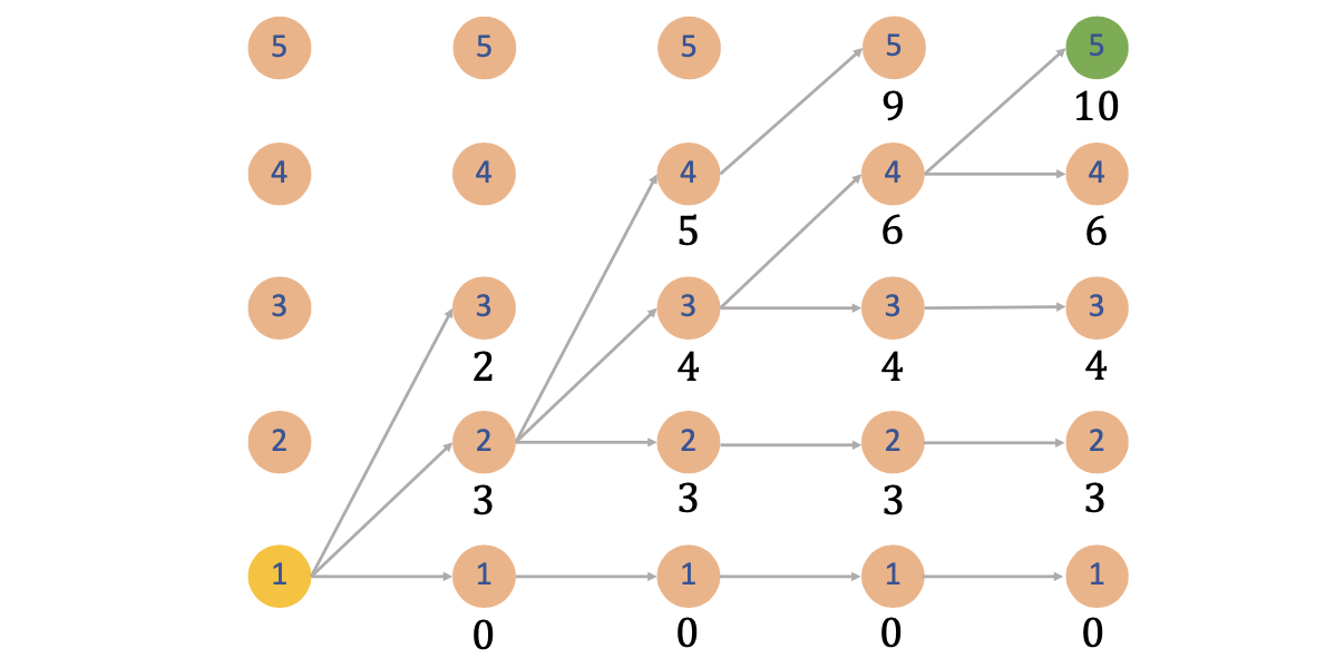
Dynamic Programming Solution

Value function:

$$T_i = \text{Earliest completion time at node } i$$

Recursion:

$$T_i = \max_{j \in \text{Pred}(i)} \left( T_j + t_{ji} \right)$$

where $\text{Pred}(i)$ is the set of direct predecessors of node $i$

Boundary condition:

$$T_1 = 0$$

Critical activity identification:
Activity $(j,i)$ is critical iff:

$$T_i = T_j + t_{ji}$$

Algorithm Properties

1. Acyclic graph guarantee:

   • Project network has no cycles → finite paths
   • Ensures $\max$ operation is well-defined

2. Critical activity property:

   • All activities on critical path are critical
   • Non-critical activities have slack time:

     $$\text{Slack} = T_i - (T_j + t_{ji})$$

Managerial insight:
Optimizing critical activities reduces total duration, non-critical activities allow resource flexibility