SDSC6012 Course 1-Introduction

#sdsc6012

English / 中文

Time Series Definition

Core Concepts

• A time series is a sequence of data points indexed in chronological order.

• Application Areas:

  • Economics: Daily stock prices, GDP, monthly unemployment rate
  • Social Sciences: Population, birth rate, enrollment rate
  • Epidemiology: Number of flu cases, mortality rate
  • Medicine: Blood pressure monitoring, fMRI data
  • Natural Sciences: Global temperature, monthly sunspot observations

Supplementary Note: Time series are observational records of real-world dynamic processes, with the core feature being that data points are ordered by timestamps.

Time Series Analysis Objectives

Analytical Significance

1. Description and Explanation: Understanding sequence generation mechanisms (e.g., trends/seasonality)

   Example: Analyzing long-term warming trends in temperature series

2. Forecasting: Predicting future values

   Example: Forecasting next quarter’s unemployment rate

3. Control: Evaluating the impact of intervention measures

   Example: Assessing the effect of monetary policy on unemployment rate

4. Hypothesis Testing: Verifying theoretical models

   Example: Testing the global warming hypothesis

Time Series Models

Basic Decomposition Model

$$x_t = m_t + s_t + e_t$$

Formula Explanation:

• $x_t$: Observed value at time $t$
• $m_t$: Trend component (long-term change trend)
• $s_t$: Seasonal component (periodic change pattern)
• $e_t$: Residual component (random fluctuation/noise)

Stochastic Process Perspective

• A time series is one realization of a stochastic process $\{x_t\}$

  Supplementary Note:

  • Stochastic process = “Natural law” generating the sequence (theoretical model)
  • Time series = Actual observed specific data (real-world record)
  • Example: Daily 3PM temperature records are a time series; temperature change patterns are a stochastic process

White Noise

Strict Definition

White noise is a stochastic process $w_t$ satisfying three conditions:

1. Zero mean: $E(w_t) = 0$

2. Constant variance: $\text{Var}(w_t) = \sigma_w^2$

3. No autocorrelation: $\text{Corr}(w_t, w_{t+k}) = 0 \ (k \neq 0)$

Mathematical Representation

$$w_t \sim \text{wn}(0, \sigma_w^2)$$

Key Properties:

• No exploitable patterns (completely random)
• Past values do not affect future values (memoryless)

Gaussian White Noise

• Special form: $w_t$ follows a normal distribution

• Cumulative distribution function:

$$P(w_t < c_t) = \Phi(c_t) = \frac{1}{\sqrt{2\pi}} \int_{-\infty}^{c_t} e^{-w^2/2} dw$$

Stationary and Non-Stationary Time Series

Core Definition

• Stationary time series: Statistical properties (e.g., mean, variance) do not change over time; series behavior is time-independent.

• Non-stationary time series: Statistical properties change over time; series behavior strongly depends on time.

Supplementary Note: The stable statistical properties of stationary series allow historical patterns to be used for future forecasting (e.g., the pattern “if the previous value is high, the next value decreases” remains applicable).

Problems and Advantages

• Non-stationary series problem: Continuously changing statistical properties may render past patterns completely invalid in the future (e.g., mean is 100 today but 110 tomorrow).

• Stationary series advantage: Fixed mean and variance ensure consistent behavioral patterns, enabling reliable forecasting.

Example: Ice Cream Sales (Non-Stationarity)

Data Characteristics

• Sales peak in summer (July-August) and trough in winter (December-January), forming repeating peak-valley patterns.

• Since sales strongly correlate with time, it is a non-stationary series.

Stationarization Method: Seasonal Differencing

$$\nabla_{365} x_t = x_t - x_{t-365}$$

Formula Explanation:

• $\nabla_{365}$: Differencing operator for a 365-day cycle
• $x_t$: Sales on day $t$ of the current year
• $x_{t-365}$: Sales on the same day of the previous year
  Operational Meaning: Computes “current year sales minus previous year sales” to eliminate fixed annual seasonal effects.

Moving Average

Purpose

Smoothing data, removing random noise, highlighting long-term trends.

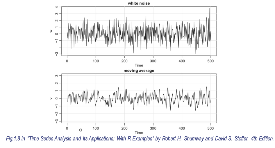
Calculation Principle

$k$-period moving average:

$$\text{MA}_t = \frac{1}{k} \sum_{i=0}^{k-1} x_{t-i}$$

Calculation Example

Original series: $[100, 102, 101, 105, 103]$

3-day moving average:

• $t=3$: $\frac{100 + 102 + 101}{3} = 101$

• $t=4$: $\frac{102 + 101 + 105}{3} \approx 102.67$

• $t=5$: $\frac{101 + 105 + 103}{3} = 103$

Output series: $[-, -, 101, 102.67, 103]$

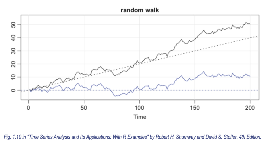
Random Walk with Drift

Basic Model

$$x_t = \delta + x_{t-1} + \omega_t$$

Formula Explanation:

• $x_t$: Value at time $t$
• $\delta$: Drift term (constant)
• $\omega_t$: White noise (mean 0, constant variance)

Model Derivation

Recursive expansion:

$$\begin{align*} x_t &= \delta + x_{t-1} + \omega_t \\ &= \delta + (\delta + x_{t-2} + \omega_{t-1}) + \omega_t \\ &= 2\delta + x_{t-2} + \omega_{t-1} + \omega_t \\ &\ \ \vdots \\ &= \delta \cdot t + \sum_{j=1}^{t} \omega_j \end{align*}$$

Physical Interpretation

Analogy:

• Random walk ($\delta=0$): A drunkard with random step directions (determined by coin toss)
• Drift term ($\delta \neq 0$): The drunkard is gently pulled northward by a rope ($\delta$ is the pulling force)
• Overall path: Northward pull ($\delta t$) + random steps ($\sum \omega_j$)

Differenced Form

$$\nabla x_t = x_t - x_{t-1} = \delta + \omega_t$$

Key Conclusion: After differencing, it transforms into white noise with a constant term ($\delta$), making the series stationary.

Signal and Noise

Model: $x_t = A\cos(2\pi\omega t + \Phi) + w_t$

This model indicates that the observed time series consists of an underlying signal (e.g., seasonal component $A\cos(2\pi\omega t + \Phi)$) and superimposed noise ($w_t$). The goal of analysis is to extract the signal from the noise.

Measures of Dependence

Mean Function

Describes the average level of the time series at any time $t$.

$$\mu_t = E(x_t) = \int_{-\infty}^{\infty} x f_t(x) dx \quad \text{(provided it exists)}$$

Examples:

1. For moving average $v_t = \frac{1}{3}(w_{t-1} + w_t + w_{t+1})$, $E(v_t) = 0$.

2. For random walk with drift $x_t = \delta t + \sum_{j=1}^{t} w_j$, $E(x_t) = \delta t$.

3. For signal-containing series $x_t = A\cos(2\pi\omega t + \phi) + w_t$, $E(x_t) = A\cos(2\pi\omega t + \phi)$.

Autocovariance Function

The autocovariance function quantifies the linear dependence between current and past values in a time series, reflecting internal dynamic dependencies. The core question is: Can changes in a variable at one time be predicted by changes at another time?

Definition:

$$\gamma(s, t) = \operatorname{Cov}(x_s, x_t) = E\left[(x_s - \mu_s)(x_t - \mu_t)\right]$$

• Measures linear dependence between different time points $s$ and $t$ in the same series.

• $\gamma(s, t) = 0$ indicates no linear relationship between $x_t$ and $x_s$.

• When $s = t$, $\gamma(t, t) = \operatorname{Var}(x_t)$.

Examples:

1. White noise $\{w_t\}$:

   $$\gamma(s, t) = \operatorname{cov}(w_s, w_t) = \begin{cases}\sigma_{w}^{2} & s=t \\ 0 & s\neq t \end{cases}$$

2. 3-term moving average $v_t = \frac{1}{3}(w_{t-1} + w_t + w_{t+1})$:

   $$\gamma(s, t) = \begin{cases} \frac{3}{9}\sigma_{w}^{2} & s=t, \\ \frac{2}{9}\sigma_{w}^{2} & |s-t|=1, \\ \frac{1}{9}\sigma_{w}^{2} & |s-t|=2, \\ 0 & |s-t|>2 \end{cases}$$

3. Random walk $x_t = \sum_{j=1}^{t} w_j$:

   $$\gamma(s, t) = \operatorname{cov}(x_s, x_t) = \operatorname{cov}\left(\sum_{j=1}^{s} w_j, \sum_{k=1}^{t} w_k\right) = \min\{s, t\}\sigma_{w}^{2}$$