SDSC6012 Course 4-Autoregressive models

#sdsc6012

English / 中文

Stationarity

Strict Stationarity

A time series $\{x_t\}$ is strictly stationary if and only if for any $k$, any time points $t_1, t_2, \ldots, t_k$, and any time shift $h$, we have:

$$P\{x_{t_1} \leq c_1, \ldots, x_{t_k} \leq c_k\} = P\{x_{t_1+h} \leq c_1, \ldots, x_{t_k+h} \leq c_k\}$$

Core Meaning: Strict stationarity implies that the complete probability distribution of the time series does not change over time. Regardless of which time window is selected, its joint distribution properties remain unchanged. This allows statistical quantities obtained from a single time series sample to be valid estimates of population properties.

Weak Stationarity

A time series $\{x_t\}$ is weakly stationary if it satisfies:

1. $\mu_t = E[x_t]$ is constant (independent of time $t$)

2. $\gamma(t+h, t) = \operatorname{Cov}(x_{t+h}, x_t)$ depends only on the time lag $h$, and not on the specific time point $t$

Practical Meaning: Weak stationarity only requires the first moment (mean) and second moments (variance, covariance) to be stable, and does not require the complete probability distribution to be stable. This makes “prediction” possible because the statistical properties do not change over time.

Feature	Strict Stationarity	Weak Stationarity
Core Definition	For any set of time points t₁, t₂, …, tₙ and any time shift k, the joint distribution satisfies: F_{X_{t₁},…,X_{tₙ}}(x₁,…,xₙ) = F_{X_{t₁+k},…,X_{tₙ+k}}(x₁,…,xₙ) (All finite-dimensional joint distributions remain unchanged)	1. E[Xₜ] = μ (constant) 2. Cov(Xₜ, Xₜ₊ₖ) = γ(k) (depends only on lag k, not on time t)
Mean	Not explicitly required, but as a corollary, if it exists, it must be constant: E[Xₜ] = μ (constant for all t)	Explicitly required: E[Xₜ] = μ (constant for all t)
Variance	Not explicitly required, but as a corollary, if it exists, it must be constant: Var(Xₜ) = σ² (constant for all t)	Not directly required, but since covariance depends only on lag, variance is naturally constant: Var(Xₜ) = γ(0) (constant)
Focus	Complete probability distribution	Only the first two moments (mean, variance, covariance)

Properties of the Autocovariance Function

For a stationary process, the autocovariance function $\gamma(h)$ satisfies:

1. $\gamma(0) \geq 0$ (variance is non-negative)

2. $|\gamma(h)| \leq \gamma(0)$ (absolute autocovariance does not exceed variance)

3. $\gamma(h) = \gamma(-h)$ (even function)

Autocorrelation Function (ACF)

$$\rho(h) = \frac{\gamma(h)}{\gamma(0)} = \frac{\operatorname{Cov}(x_t, x_{t+h})}{\operatorname{Var}(x_t)}=Corr(x_{t+h}, x_t)$$

Note:
$\gamma(h)$ is the autocovariance function, i.e., $Cov(X_t, X_{t+h})$.
$\gamma(0)$ is the variance of the time series, i.e., $Var(X_t)$.

Standardization Meaning: By dividing by the variance $\gamma(0)$, the ACF is constrained to the range $[-1, 1]$, facilitating comparison of correlation strengths between different time series.

Time Series Analysis

Basic Concept Review

For time series observations $x_{1}, x_{2}, \ldots, x_{n}$, we define the following sample statistics:

• Sample Mean:

  $$\bar{x} = \frac{1}{n} \sum_{t=1}^{n} x_{t}$$

  Represents the average level of the time series.

• Sample Autocovariance Function:
  For lag $h$ (where $h = 0, 1, 2, \ldots$),

  $$\hat{\gamma}(h) = \frac{1}{n} \sum_{t=1}^{n-h} (x_{t} - \bar{x})(x_{t+h} - \bar{x})$$

  Measures the covariance between observations separated by $h$ time points. When $h=0$, it is the sample variance.

• Sample Autocorrelation Function (sample ACF):

  $$\hat{\rho}(h) = \frac{\hat{\gamma}(h)}{\hat{\gamma}(0)}$$

  Represents the standardized autocovariance, ranging from $[-1, 1]$, used to measure linear correlation.

Simple Example Calculation

Assume a simple time series sample: $[2, 4, 6, 8]$, i.e., $n = 4$.

• Calculate Sample Mean:

  $$\bar{x} = \frac{2 + 4 + 6 + 8}{4} = 5$$

• Calculate $\hat{\gamma}(0)$ (Sample Variance):

  $$\begin{align*} \hat{\gamma}(0) & = \frac{1}{4} \sum_{t=1}^{4} (x_t - 5)^2 \\ & = \frac{1}{4} \left[ (2-5)^2 + (4-5)^2 + (6-5)^2 + (8-5)^2 \right] \\ & = \frac{1}{4} (9 + 1 + 1 + 9) \\ & = 5 \end{align*}$$

• Calculate $\hat{\gamma}(1)$ (Autocovariance at Lag 1):

  $$\begin{align*} \hat{\gamma}(1) & = \frac{1}{4} \sum_{t=1}^{3} (x_t - 5)(x_{t+1} - 5) \\ & = \frac{1}{4} \left[ (2-5)(4-5) + (4-5)(6-5) + (6-5)(8-5) \right] \\ & = \frac{1}{4} \left[ (-3)(-1) + (-1)(1) + (1)(3) \right] \\ & = \frac{1}{4} (3 - 1 + 3) \\ & = 1.25 \end{align*}$$

Asymptotic Properties of White Noise Processes

For a white noise process $w_t$, if $E[w_t^4] < \infty$, then the sample ACF $\hat{\rho}(h)$ satisfies:

• $\hat{\rho}(h) \sim N(0, 1/n)$ asymptotic distribution

• For $h \neq 0$, $\hat{\rho}(h)$ is asymptotically normally distributed with mean 0 and variance $1/n$

Practical Meaning: In large samples, we can use the normal distribution to test the significance of ACF values, determining whether a particular lag has true statistical significance.

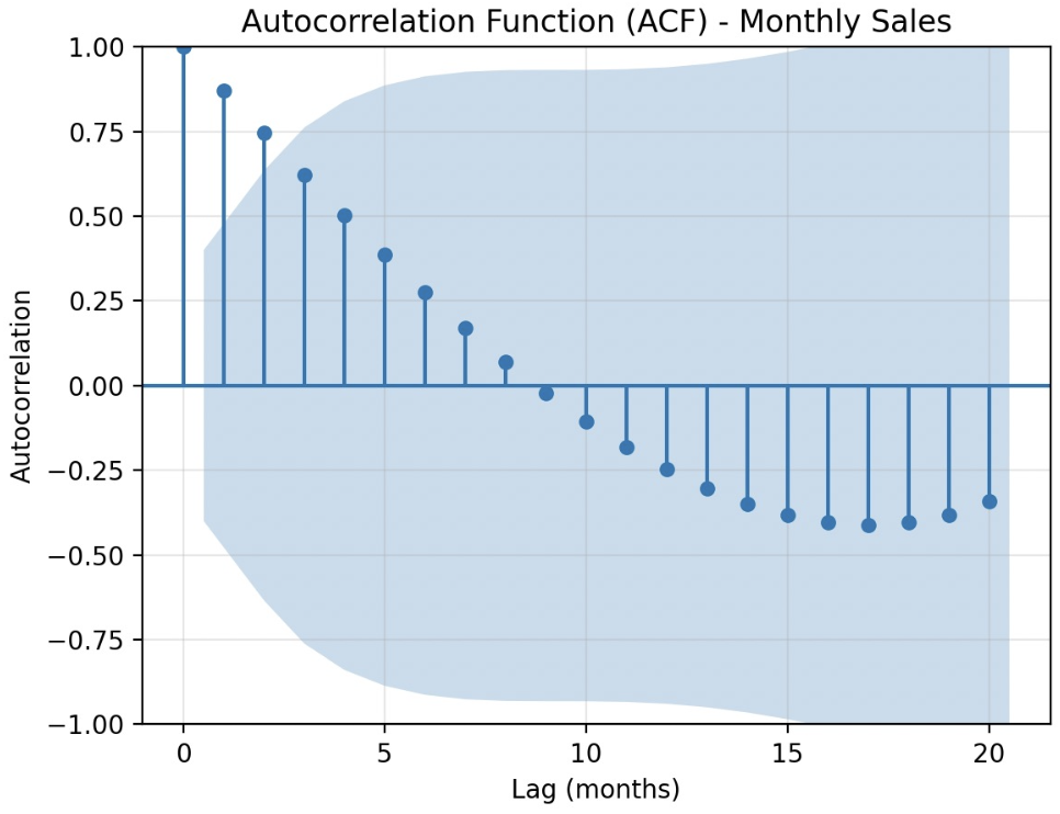
Company Sales Data Case Analysis

Sales data (24 months):

$$\begin{align*} \text{Sales} = [ & 100, 112, 125, 138, 150, 163, \\ & 177, 190, 205, 220, 235, 250, \\ & 265, 281, 298, 315, 333, 351, \\ & 370, 389, 409, 430, 451, 473] \end{align*}$$

• Using Python for ACF Analysis:
  Code uses the statsmodels library to plot the ACF and calculate ACF values.

  • The plot_acf function generates the autocorrelation plot, and the acf function calculates specific values.
  • Output includes ACF values for the first 10 lags, e.g., Lag0:1.0000, Lag1: high value (due to growth trend), etc.

Time Series Operators

Backshift Operator

• Definition: $B x_t = x_{t-1}$

• Multiple Applications: $B^k x_t = x_{t-k}$ (shift backward by k time units)

Example:
Assume a time series: $x_1 = 5, x_2 = 8, x_3 = 6, x_4 = 9, x_5 = 7$

• $B x_3 = x_2 = 8$

• $B^2 x_4 = x_2 = 8$

• $B x_5 = x_4 = 9$

Forward-shift Operator

• Definition: $F x_t = x_{t+1}$

• Multiple Applications: $F^k x_t = x_{t+k}$ (shift forward by k time units)

• Relationship: $F = B^{-1}$, $x_t = B^{-1} x_{t-1}$

Example:
Using the same series: $x_1 = 5, x_2 = 8, x_3 = 6, x_4 = 9, x_5 = 7$

• $F x_2 = x_3 = 6$

• $F^2 x_1 = x_3 = 6$

• $F x_4 = x_5 = 7$

First Difference Operator (Eliminating Linear Trend)

Definition and Calculation

• Definition: $\nabla x_t = (1 - B) x_t$

• Calculation: $\nabla x_t = x_t - x_{t-1}$ (calculate the change between consecutive observations)

Working Principle Analysis

1. Current Value Component: $1 \cdot x_t = x_t$

2. Previous Value Component: $-B x_t = -x_{t-1}$

3. Combined Effect: $(1 - B) x_t = x_t - x_{t-1}$

Complete Calculation Example

Time(t)	Observation(xₜ)	Difference Calculation Process	Difference Result(∇xₜ)
1	10	-	Missing
2	12	12 - 10 = 2	2
3	14	14 - 12 = 2	2
4	16	16 - 14 = 2	2
5	18	18 - 16 = 2	2

Result Analysis: The differenced series is [Missing, 2, 2, 2, 2], constant difference values indicate the original series has a perfect linear trend.

d-th Difference Operator (Eliminating Higher-Order Trends)

• Definition: $\nabla^d = (1 - B)^d$

• Application: Used to eliminate polynomial trends; d-th difference can eliminate a d-th degree polynomial trend.

Empirical Evidence of Trend Elimination by Difference Operators

Mathematical Proof of Linear Trend Elimination

When the time series has a linear trend: $x_t = \beta_0 + \beta_1 t + y_t$

First Difference Calculation Process:

$$\begin{aligned} \nabla x_t &= x_t - x_{t-1} \\ &= (\beta_0 + \beta_1 t + y_t) - (\beta_0 + \beta_1 (t-1) + y_{t-1}) \\ &= \beta_1 + y_t - y_{t-1} \end{aligned}$$

Conclusion: The linear trend term $\beta_1 t$ is completely eliminated, leaving only the constant term $\beta_1$ and the difference of the stationary component.

Mathematical Proof of Quadratic Trend Elimination

When the time series has a quadratic trend: $x_t = \beta_0 + \beta_1 t + \beta_2 t^2 + y_t$

First Difference Result:

$$\nabla x_t = \beta_1 - \beta_2 + 2\beta_2 t + y_t - y_{t-1}$$

Second Difference Calculation:

$$\begin{aligned} \nabla^2 x_t &= \nabla(\nabla x_t) \\ &= (2\beta_2 t + \beta_1 - \beta_2 + y_t - y_{t-1}) - (2\beta_2 (t-1) + \beta_1 - \beta_2 + y_{t-1} - y_{t-2}) \\ &= 2\beta_2 + y_t - 2y_{t-1} + y_{t-2} \end{aligned}$$

Conclusion: The quadratic trend is completely eliminated, leaving only the constant term $2\beta_2$ and the second difference of the stationary component.

Linear Process

Definition

A time series $\{x_t\}$ is called a linear process if it can be expressed as:

$$x_t = \mu + \sum_{j=-\infty}^{\infty} \psi_j w_{t-j}$$

where:

• $\{w_t\} \sim \operatorname{wn}(0, \sigma_w^2)$ (white noise process)

• $\mu$ is the mean of the process

• $\psi_j$ are weight coefficients satisfying absolute summability: $\sum_{j=-\infty}^{\infty} |\psi_j| < \infty$

Component Analysis

• Causal Part: $j \geq 0$, indicating the current value depends on present and past shocks

• Non-causal Part: $j < 0$, indicating the current value depends on future shocks

• Absolute Summability Condition: $\sum |\psi_j| < \infty$ ensures the weight coefficients eventually decay to zero: $\lim_{|j|\to\infty} |\psi_j| = 0$

Relationship with AR Models

Important Conclusion: All stationary AR models are special cases of linear processes, but not all linear processes are AR models. AR models store “memory” in their own past values, while linear processes express through weighted sums of white noise shocks.

Linear Processes and Autoregressive Models (AR)

Core Relationship

The relationship between linear processes and autoregressive models can be summarized as:

“All (stationary) AR models are linear processes, but not all linear processes are AR models.”

Example Illustration

• Linear Process: Like a broad “model family”, containing various types of models

• AR Model: A “specific and widely used member” of this family

Key Difference:

• AR models store “memory” in their own historical values ($x_{t-1}, x_{t-2}, ...$)

• Define the current value through linear combinations of past observations

Autoregressive Models (AR)

Intuitive Understanding

The core idea of AR models: the current value $x_t$ of a time series can be explained by a linear combination of its past $p$ values.

Mathematical Expression:

$$x_t = \phi_1 x_{t-1} + \phi_2 x_{t-2} + \cdots + \phi_p x_{t-p} + w_t$$

where:

• $\phi_1, \phi_2, ..., \phi_p$ are autoregressive coefficients

• $w_t$ is the white noise term (random shock at the current time)

Examples of AR Models of Different Orders

AR(1) Model (First-Order Autoregressive)

Model Form:

$$Today's Temperature = \phi_1 \times Yesterday's Temperature + Random Shock$$

Practical Meaning: Only considers the effect of yesterday on today

Specific Example:
Assume $\phi_1 = 0.8$, then:

$$Today's Temperature = 0.8 \times Yesterday's Temperature + Random Fluctuation$$

AR(2) Model (Second-Order Autoregressive)

Model Form:

$$Today's Temperature = \phi_1 \times Yesterday's Temperature + \phi_2 \times Day Before Yesterday's Temperature + Random Shock$$

Practical Meaning: Considers the combined influence of yesterday and the day before yesterday

Specific Example:
Assume $\phi_1 = 0.6$, $\phi_2 = 0.3$, then:

$$Today's Temperature = 0.6 \times Yesterday's Temperature + 0.3 \times Day Before Yesterday's Temperature + Random Fluctuation$$

Practical Application Example

Stock Market Price Prediction

Assume a stock’s daily closing price follows an AR(2) model:

$$Today's Stock Price = 0.6 \times Yesterday's Price + 0.3 \times Day Before Yesterday's Price + Random Fluctuation$$

This means:

• 60% of today’s price is influenced by yesterday’s price

• 30% is influenced by the day before yesterday’s price

• The remaining 10% comes from random fluctuations

Applicable Scenario: AR models are suitable for data with trends, i.e., where the current value depends on past observations.

Operator Notation

Backshift Operator

• Definition: $B x_t = x_{t-1}$

• Multiple Applications:

  • $B^2 x_t = x_{t-2}$ (shift backward by 2 steps)
  • $B^p x_t = x_{t-p}$ (shift backward by p steps)

Operator Form of AR Models

Convert the AR(p) model:

$$x_t = \phi_1 x_{t-1} + \phi_2 x_{t-2} + \cdots + \phi_p x_{t-p} + w_t$$

to:

$$(1 - \phi_1 B - \phi_2 B^2 - \cdots - \phi_p B^p) x_t = w_t$$

Define the autoregressive operator:

$$\phi(B) = 1 - \phi_1 B - \phi_2 B^2 - \cdots - \phi_p B^p$$

Finally, obtain the concise form:

$$\phi(B) x_t = w_t$$

Operator Interpretation

$\phi(B)$ is not just an abbreviation; it represents a system or filter:

• Input: Original time series $x_t$

• System: $\phi(B)$ (defined by parameters $\phi_1, \phi_2, ..., \phi_p$)

• Output: White noise $w_t$

Meaning: If we filter the original series through this $\phi(B)$ system, all predictable patterns that can be captured by past values will be removed, ultimately outputting pure random white noise.

Detailed Analysis of AR(1) Model

Model Form

$$x_t = \phi x_{t-1} + w_t$$

Solution Process

By successive substitution:

$$x_t = \phi x_{t-1} + w_t = \phi(\phi x_{t-2} + w_{t-1}) + w_t = \phi^2 x_{t-2} + \phi w_{t-1} + w_t$$

Continue this process n times:

$$x_t = \phi^n x_{t-n} + \sum_{j=0}^{n-1} \phi^j w_{t-j}$$

Operator Solution

Using the backshift operator: $(1 - \phi B) x_t = w_t$

Apply the inverse operator (valid when $|\phi| < 1$):

$$x_t = (1 - \phi B)^{-1} w_t = \sum_{j=0}^{\infty} \phi^j B^j w_t = \sum_{j=0}^{\infty} \phi^j w_{t-j}$$

Causality and Stationarity

Causal Process

A time series process is called causal if its current value depends only on:

• Present and past inputs/shock processes

• Does not depend on future values

Causality Condition for AR(1) Model

The AR(1) process $x_t = \phi x_{t-1} + w_t$ is causal if and only if:

Condition 1: $|\phi| < 1$

Condition 2: The root $z_1$ of the polynomial $\phi(z) = 1 - \phi z$ satisfies $|z_1| > 1$

When $|\phi| < 1$: The process can be expressed as $x_t = \sum_{j=0}^{\infty} \phi^j w_{t-j}$, depending only on past and present noise.

Non-causal Case

When $|\phi| > 1$, the process is non-causal, depending on future noise:

$$x_t = -\sum_{j=1}^{\infty} \phi^{-j} w_{t+j}$$

Stationarity Condition for AR(p) Models

An AR(p) model has a stationary solution if and only if all roots of the autoregressive characteristic polynomial:

$$\phi(z) = 1 - \phi_1 z - \phi_2 z^2 - \cdots - \phi_p z^p = 0$$

lie outside the unit circle (i.e., the modulus of all roots is greater than 1).

Example: Checking Causality

Example 1: AR(2) Model

Consider the model: $x_t = 1.5x_{t-1} - 0.5x_{t-2} + w_t$

Characteristic polynomial: $\phi(z) = 1 - 1.5z + 0.5z^2$

Solve the equation: $1 - 1.5z + 0.5z^2 = 0$
Roots: $z_1 = 1$, $z_2 = 2$

Since $|z_1| = 1$ (on the unit circle), the process is not causal.

Example 2: AR(2) Model

Consider the model: $x_t = 0.5x_{t-1} + 0.2x_{t-2} + w_t$

Characteristic polynomial: $\phi(z) = 1 - 0.5z - 0.2z^2$

Solve the equation to get roots: $z_1 \approx -1.35$, $z_2 \approx 3.70$

Since $|z_1| \approx 1.35 > 1$ and $|z_2| \approx 3.70 > 1$, the process is causal.