SDSC6015 Course 1-Introduction / Preliminaries of Stochastic Optimization

#sdsc6015

English / Chinese

Course Introduction and Preliminary Stochastic Optimization

---

Main Problem

Given labeled training data $(x_1, y_1), \dots, (x_n, y_n) \in \mathbb{R}^d \times \mathcal{Y}$,
find weights $\theta$ to minimize:

$$\min_{\theta} f(\theta) = \frac{1}{n} \sum_{i=1}^{n} \ell(\theta, (x_i, y_i)), \quad n \text{ extremely large}$$

Objective: Quantify model prediction error through the loss function $\ell$ and optimize parameters $\theta$.

Supplementary Notes

Mathematical Notation Explanation:

• $\theta \in \mathbb{R}^m$: Parameter vector to optimize (e.g., weights in linear models, neural network parameters)

• $\ell(\theta, (x_i, y_i))$: Loss function, quantifying the discrepancy between model prediction $\hat{y}_i = g_\theta(x_i)$ and true label $y_i$

• $\frac{1}{n} \sum_{i=1}^n$: Empirical risk, representing the average loss over the training set

Practical Significance:

This optimization problem is called Empirical Risk Minimization (ERM):

• Core Idea: Generalize the model to new data by minimizing average loss on the training set
• Challenge: High computational cost for gradient calculation when $n$ is extremely large
• Solution: Stochastic optimization algorithms (e.g., SGD) approximate gradients using subsets of data per iteration

---

Soft Margin Support Vector Machine (SVM)

$$\min_{w,b} \left\{ \frac{1}{n} \sum_{i=1}^{n} \max\left(0, 1 - y_i (w^\top x_i - b)\right) + \lambda \|w\|^2 \right\}$$

• $x_i$: Feature vector

• $y_i \in \{-1, 1\}$: Class label

• $\lambda > 0$: Regularization coefficient

• $w, b$: Parameters to learn

Hinge Loss: $\max(0, 1 - y_i (w^\top x_i - b))$ penalizes misclassification.
Regularization: $\lambda \|w\|^2$ controls model complexity to prevent overfitting.

Supplementary Notes

Mathematical Derivation:

1. Origin of Hinge Loss:

   • Ideal constraint $y_i(w^\top x_i - b) \geq 1$ (all samples correctly classified with margin ≥1)
   • Introduce slack variables $\xi_i \geq 0$ to allow constraint violation: $y_i(w^\top x_i - b) \geq 1 - \xi_i$
   • Minimize violation degree $\sum \xi_i$ → $\max(0, 1 - y_i(w^\top x_i - b))$

   Geometric Interpretation: Distance from sample to decision boundary $d = \frac{|w^\top x_i - b|}{\|w\|}$, penalized when $d < \frac{1}{\|w\|}$

2. Derivation of Regularization Term:

   • Margin size $M = \frac{2}{\|w\|}$
   • Maximizing margin is equivalent to minimizing $\|w\|^2$ (since $\arg\max M = \arg\min \|w\|$)

   Practical Meaning: $\lambda$ balances classification error and model complexity

   • $\lambda \to 0$: Allows more misclassification (large margin)
   • $\lambda \to \infty$: Strict classification (small margin)

Extended Notation Explanation:

• $w^\top x_i - b = 0$: Decision hyperplane (boundary separating classes)

• $\frac{w}{\|w\|}$: Normal vector direction (determines classification direction)

• $b$: Intercept term (adjusts hyperplane position)

Example:
In 2D space:

• Decision boundary is line $w_1x_1 + w_2x_2 - b = 0$

• Positive class ($y_i=1$) on one side, negative class ($y_i=-1$) on the other

• Hinge loss activates only when samples enter the “margin zone” (gray area)

---

Example: Image Denoising

Total Variation Denoising Model:

$$\min_{X} \sum_{(i,j) \in P} |X_{ij} - O_{ij}|^2 + \lambda \cdot TV(X)$$

• $X$: Image matrix to recover

• $O$: Noisy observed image

• $P$: Set of observed pixel indices

• $TV(X)$: Total variation regularization term:

  $$TV(X) = \sum_{i,j} |X_{i+1,j} - X_{ij}| + |X_{i,j+1} - X_{ij}|$$

Data Fidelity Term: $\sum |X_{ij} - O_{ij}|^2$ ensures recovered image resembles observations.
Smoothness Constraint: $TV(X)$ promotes piecewise smoothness by penalizing adjacent pixel differences.

Supplementary Notes

Mathematical Derivation:

1. Physical Meaning of $TV(X)$:

   • $|X_{i+1,j} - X_{ij}|$ computes vertical gradient (intensity difference with lower neighbor)
   • $|X_{i,j+1} - X_{ij}|$ computes horizontal gradient (intensity difference with right neighbor)

   Core Idea: Natural images exhibit “piecewise smooth” properties (similar adjacent pixels), while noise disrupts continuity

2. Optimization Objective Decomposition:

   • Data Fidelity Term: Minimize $\|X - O\|_F^2$ (squared Frobenius norm) → Maintain similarity to observed image
   • Regularization Term: Minimize image gradient $\|\nabla X\|_1$ (L1 norm of gradient vector) → Promote smoothness

   $\lambda$ controls smoothness strength: $\lambda \uparrow$ → Smoother but may blur details

Extended Notation Explanation:

• $X_{ij} \in [0,255]$: Pixel intensity (grayscale value) at position $(i,j)$

• $\nabla X = \begin{bmatrix} X_{i+1,j}-X_{ij} \\ X_{i,j+1}-X_{ij} \end{bmatrix}$: Discrete gradient operator

• L1 norm $\|\nabla X\|_1$: More robust to noise (compared to L2 norm)

Practical Significance:

• Medical Imaging: Remove Gaussian noise in CT scans while preserving organ boundaries

• Satellite Imagery: Eliminate cloud interference and restore surface textures

• Comparison with Gaussian Filtering: TV denoising preserves edges (e.g., building contours), while Gaussian filtering blurs edges

Example:
Assume 2×2 noisy image $O = \begin{bmatrix} 50 & 100 \\ 30 & 80 \end{bmatrix}$:

• Compute $TV(O) = |50-30| + |50-100| + |30-80| + |100-80| = 20+50+50+20=140$

• Denoised image $X$ has significantly reduced $TV(X)$ (e.g., 40) while $|X-O|^2$ remains small

---

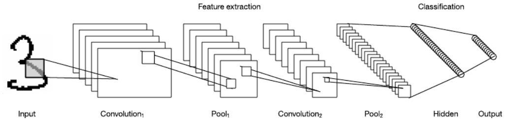
Example: Neural Networks

Convolutional Neural Network (CNN):

$$\min_{w,b} f(w,b) = \frac{1}{n} \sum_{i=1}^{n} \ell(w, b, (x_i, y_i))$$

where

$$\ell(w, b, (x_i, y_i)) = \left\| w_3^\top \cdot Q(w_2^\top \cdot Q(w_1^\top x_i - b_1) - b_2) - y_i \right\|^2$$

• $Q(w)_i = \max(0, w_i)$: ReLU activation function

• $w_1, w_2, w_3$: Weight matrices

• $b_1, b_2$: Bias vectors

• $x_i$: Input data, $y_i$: Target output

ReLU Activation: $Q(\cdot)$ outputs 0 for negative inputs, introducing nonlinearity.
Hierarchical Structure: Nested transformations $w_k^\top \cdot Q(\cdot) - b_k$ model complex feature interactions.

Supplementary Notes

Mathematical Derivation:

1. Forward Propagation Process:

   • Input Layer: $x_i \in \mathbb{R}^{d_0}$ (raw input, e.g., image pixels)
   • Hidden Layer 1: $z^{(1)} = w_1^\top x_i - b_1$ (linear transformation)
     $a^{(1)} = Q(z^{(1)})$ (ReLU activation, $\max(0, z^{(1)})$)
   • Hidden Layer 2: $z^{(2)} = w_2^\top a^{(1)} - b_2$
     $a^{(2)} = Q(z^{(2)})$
   • Output Layer: $\hat{y}_i = w_3^\top a^{(2)}$ (predicted value)

   $\ell = \|\hat{y}_i - y_i\|^2$ computes squared error between prediction and true value

2. Mathematical Properties of ReLU:

   $$Q(z) = \begin{cases} z & \text{if } z > 0 \\ 0 & \text{otherwise} \end{cases}$$

   Advantages:

   • Solves vanishing gradient problem (gradient=1 in positive region)
   • Sparse activation (~50% neuron activation)

Extended Notation Explanation:

• $w_k \in \mathbb{R}^{d_{k} \times d_{k-1}}$: Weight matrix ($d_k$ = number of neurons in layer $k$)

• $b_k \in \mathbb{R}^{d_k}$: Bias vector (shifts decision boundary)

• $Q(\cdot)$: Element-wise operation (applies ReLU independently to each element)

Practical Significance:

• Feature Extraction:

  • Shallow layers learn edges/textures ($w_1$)
  • Middle layers learn parts/shapes ($w_2$)
  • Deep layers learn semantic concepts ($w_3$)

• Optimization Challenges:

  • Non-convex objective (multiple local optima)
  • Gradient computation requires backpropagation (chain rule)

Example (Digit Recognition):
Input $x_i$ is 28×28 handwritten digit image ($d_0=784$):

1. $w_1$: Convolutional kernels extract edges (output $d_1=32$ feature maps)

2. $Q$: Retains positive activations (enhances feature contrast)

3. $w_2$: Combines edges into digit components (e.g., horizontal stroke of “7”)

4. $w_3$: Combines components into digits 0-9 (output $d_3=10$)

---

Simple Numerical Example: Least Squares Regression

Problem Setup

$$\min_{x} f(x) := \frac{1}{2} \|Ax - y\|^2$$

• $A \in \mathbb{R}^{n \times d}$: Data matrix

• $y \in \mathbb{R}^{n}$: Observation vector

• $x \in \mathbb{R}^{d}$: Variable to optimize

Gradient Descent (GD) vs. Stochastic Gradient Descent (SGD)

Method	Update Rule	Gradient Calculation	Per-Step Cost
GD	$x_{t+1} = x_t - \eta \nabla f(x_t)$	$\nabla f(x) = A^\top (Ax - y)$	$O(nd)$
SGD	$x_{t+1} = x_t - \eta \nabla f_t(x_t)$	$\nabla f_t(x) = a_i^\top (a_i x - y_i)$	$O(d)$

Core Idea:

• GD uses all $n$ data points per step → High computation cost but stable convergence.
• SGD uses one random data point $(a_i, y_i)$ per step → Computationally efficient for large-scale data, but noisy convergence.

Simulation Parameters

• Data: $A = \begin{bmatrix} 1 & 2 \\ 2 & 1 \\ 1 & 1 \end{bmatrix}$, $y = \begin{bmatrix} 1.5 \\ 3.5 \\ 2.0 \end{bmatrix}$ ($n=3$, $d=2$)

• Step Size: $\eta = 0.1$

• Initial Value: $x_0 = (0, 0)$

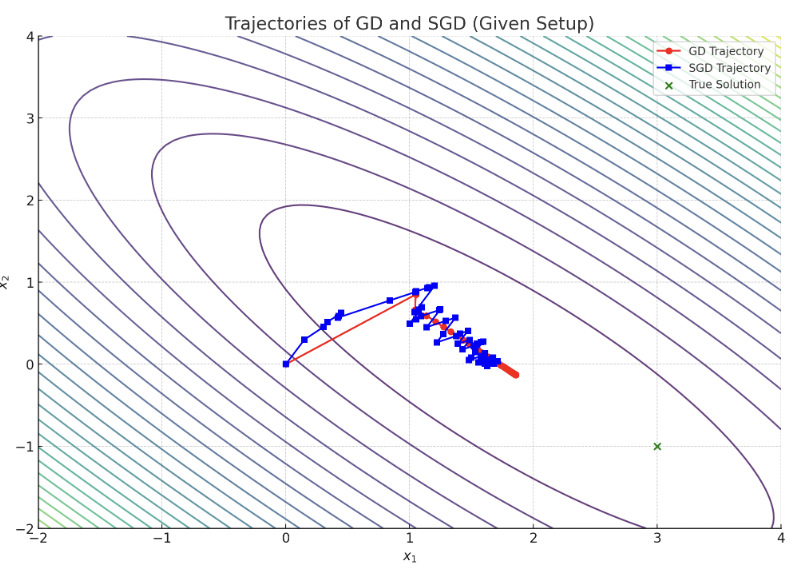
Key Takeaways

• GD: Smooth convergence but high per-iteration cost.

• SGD: Low per-step cost, practically faster convergence for large-scale problems (despite noisy path).

Preliminaries of Stochastic Optimization

---

Cauchy-Schwarz Inequality

For any vectors $u, v \in \mathbb{R}^d$:

$$|u^\top v| \leq \|u\| \|v\|$$

Notation Explanation:

• $u = \begin{pmatrix} u_1 \\ \vdots \\ u_d \end{pmatrix}$, $v = \begin{pmatrix} v_1 \\ \vdots \\ v_d \end{pmatrix}$: $d$-dimensional real column vectors

• $u^\top v = \sum_{i=1}^d u_i v_i$: Scalar product (inner product)

• $\|u\| = \sqrt{u^\top u} = \sqrt{\sum_{i=1}^d u_i^2}$: Euclidean norm

Geometric Interpretation:

• For unit vectors ($\|u\|=\|v\|=1$), equality holds iff $u=v$ or $u=-v$
• Defines vector angle $\alpha$: $\cos \alpha = \frac{u^\top v}{\|u\|\|v\|}$, satisfying $-1 \leq \cos \alpha \leq 1$

Examples for unit vectors (‖u‖=‖v‖= 1)

Equality in Cauchy-Schwarz if and only u = v or u = −v.

---

Hölder’s Inequality

For $p,q > 1$ with $\frac{1}{p} + \frac{1}{q} = 1$, and any vectors $x,y$:

$$\sum_{i=1}^n |x_i y_i| \leq \left( \sum_{i=1}^n |x_i|^p \right)^{1/p} \left( \sum_{i=1}^n |y_i|^q \right)^{1/q}$$

Related Concepts:

• $\ell_p$-norm: $\|x\|_p = \left( \sum_{i=1}^n |x_i|^p \right)^{1/p}$

• Larger $p$ gives higher weight to large components

• Cauchy-Schwarz is a special case when $p=q=2$

Core Idea: Quantify upper bounds on vector interactions via $\ell_p$ and $\ell_q$ norms.

---

Convex Sets

A set $C$ is convex iff the line segment between any two points lies within $C$:

$$\forall x,y \in C, \ \forall \lambda \in [0,1], \quad \lambda x + (1-\lambda)y \in C$$

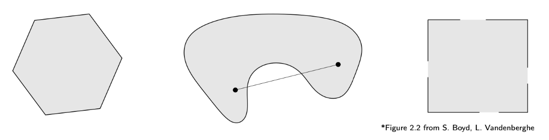
Left: Convex set
Middle: Non-convex set (segment not fully contained)
Right: Non-convex set (missing boundary points)

Properties of Convex Sets

1. Closed under intersection: Intersection of convex sets is convex

   $$\bigcap_{i \in I} C_i \text{ convex}, \quad \forall \text{ convex sets } C_i$$

2. Unique projection: For non-empty closed convex set $C$, the projection operator $P_C(x) = \arg\min\limits_{y \in C} \|y - x\|$ has a unique solution

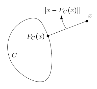
3. Non-expansiveness:

   $$\|P_C(x) - P_C(y)\| \leq \|x - y\|, \quad \forall x,y$$

---

Lipschitz Continuity

A function $f: \mathbb{R}^d \to \mathbb{R}$ is $L$-Lipschitz continuous if:

$$\|f(x) - f(y)\| \leq L\|x - y\|, \quad \forall x,y \in \mathbb{R}^d$$

Meaning of $L$: Upper bound on function change rate
Examples: $f(x) = \sqrt{x^2 + 5}$, $f(x) = \|x\|$

---

Differentiable Functions

A function $f: \mathbb{R}^d \to \mathbb{R}$ is differentiable at $x_0$ if there exists gradient $\nabla f(x_0)$ such that:

$$f(x_0 + h) \approx f(x_0) + \nabla f(x_0)^\top h$$

where $h$ is a small perturbation. If differentiable everywhere, its graph has a tangent hyperplane at every point.

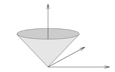
Non-Differentiable Function Example

$$f(x) = \|x\| \quad \text{(Euclidean norm)}$$

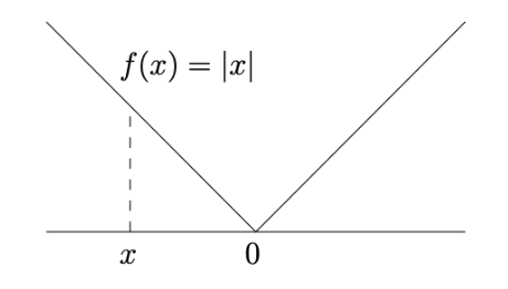
Characteristic: Non-differentiable at origin (“ice cream cone” shape)

---

L-Smoothness

A function $f: \mathbb{R}^d \to \mathbb{R}$ is $L$-smooth if:

1. $f$ is continuously differentiable (gradient $\nabla f$ exists and is continuous)

2. Gradient satisfies $L$-Lipschitz condition:

   $$\|\nabla f(x) - \nabla f(y)\| \leq L\|x - y\|, \quad \forall x,y$$

Gradient Definition:

$$\nabla f(x) = \left( \frac{\partial f}{\partial x_1}(x), \dots, \frac{\partial f}{\partial x_d}(x) \right)$$

Example: $f(x) = \frac{1}{2}\|x\|^2$ is $1$-smooth

Supplementary Notes

Mathematical Derivation:

1. Computing Lipschitz Constant:

   $$L = \sup_{x \neq y} \frac{|f(x) - f(y)|}{\|x - y\|}$$

   Maximum secant slope between any two points

2. Lipschitz Condition for Differentiable Functions:
   If $f$ differentiable, $L = \sup_{x} \|\nabla f(x)\|$

   Proof: By mean value theorem $|f(x)-f(y)| = |\nabla f(\xi)^\top (x-y)| \leq \|\nabla f(\xi)\|\|x-y\|$

Extended Notation Explanation:

• $\|x - y\|$: Euclidean distance between points in $\mathbb{R}^d$

• $L$: Lipschitz constant (upper bound on function change rate)

• $|f(x)-f(y)|$: Absolute value of function change

Practical Significance:

• Optimization Algorithm Stability:

  • In gradient descent, $L$ determines maximum step size ($\eta < 2/L$)
  • Ensures convergence (prevents oscillation or divergence)

• Neural Network Training:

  • Lipschitz constraints on weight matrices control model sensitivity
  • Enhance adversarial robustness (resist input perturbations)

Example Verification:

1. $f(x) = \|x\|$:

   $$| \|x\| - \|y\| | \leq \|x - y\| \quad (\text{triangle inequality})$$

   → $L=1$

2. $f(x) = \sqrt{x^2 + 5}$:

   $$\left| \frac{d}{dx}\sqrt{x^2+5} \right| = \frac{|x|}{\sqrt{x^2+5}} \leq 1$$

   → $L=1$

3. Non-Lipschitz Function: $f(x) = x^2$

   $$\frac{|x^2 - y^2|}{|x-y|} = |x+y| \xrightarrow{|x|,|y|\to\infty} \infty$$

   → No global Lipschitz constant

Geometric Interpretation:

• Graph of Lipschitz continuous function confined within a “slope cone”

• Vertical distance between any two points ≤ $L \times$ horizontal distance

---

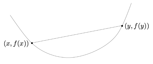
Convex Functions

---

Definition and Geometric Interpretation

A function $f: \mathbb{R}^d \to \mathbb{R}$ is convex if:

1. Domain $\text{dom}(f)$ is convex

2. Satisfies convex inequality:

   $$\forall x,y \in \text{dom}(f), \ \forall \lambda \in [0,1], \quad f(\lambda x + (1-\lambda)y) \leq \lambda f(x) + (1-\lambda)f(y)$$

Geometric Interpretation: The line segment (chord) between any two points on the graph lies above the graph.

Supplementary Notes

Mathematical Notation Explanation:

• $\lambda \in [0,1]$: Interpolation parameter, controlling linear combination ratio

• $\lambda x + (1-\lambda)y$: Convex combination, representing a point on the segment connecting $x$ and $y$

• $f(\lambda x + (1-\lambda)y)$: Function value at convex combination point

• $\lambda f(x) + (1-\lambda)f(y)$: Linear interpolation between $f(x)$ and $f(y)$

Key Property Derivation:

Convex inequality is equivalent to:

$$\frac{f(y) - f(x)}{\|y - x\|} \geq \frac{f(z) - f(x)}{\|z - x\|}, \quad \forall z \in [x,y]$$

Meaning the average growth rate is non-decreasing in any interval $[x,y]$

Practical Significance:

• Optimization Advantage: Local minima of convex functions are global minima

• Economic Decisions: Model diminishing marginal returns (e.g., production cost functions)

• Physical Systems: Spring potential $f(x) = \frac{1}{2}kx^2$ is convex ($k>0$)

Geometric Properties:

1. Chord Above Graph:

   • For any $x,y$, the segment connecting $(x,f(x))$ and $(y,f(y))$
   • Always lies above the function graph $z = f(\lambda x + (1-\lambda)y)$

2. No Local Dips:

   • Function curve has no “bowl-shaped” dips (e.g., $f(x) = -x^2$)
   • For twice differentiable functions, equivalent to $\nabla^2 f(x) \succeq 0$ (Hessian positive semi-definite)

Example Verification:

1. Convex Function: $f(x) = x^2$

   $$f(\lambda x + (1-\lambda)y) = [\lambda x + (1-\lambda)y]^2$$

   $$\lambda f(x) + (1-\lambda)f(y) = \lambda x^2 + (1-\lambda)y^2$$

   Difference: $\lambda(1-\lambda)(x-y)^2 \geq 0$ → Satisfies convex inequality

2. Non-Convex Function: $f(x) = \sin(x)$ (on $[0,2\pi]$)

   Take $x=0, y=2\pi, \lambda=0.5$:
   $f(0.5×0 + 0.5×2\pi) = \sin(\pi) = 0$
   $0.5\sin(0) + 0.5\sin(2\pi) = 0$
   But at $x=\pi/2$, $f(\pi/2)=1 > 0$ → Violates convex inequality

Metaphorical Understanding:

Imagine convex functions as “valleys”:

• Cable car line (chord) between any two points stays above valley floor (function graph)
• Water droplets sliding down converge to the lowest point (global optimum)

---

Common Convex Function Examples

1. Linear Function: $f(x) = a^\top x$

2. Affine Function: $f(x) = a^\top x + b$

3. Exponential Function: $f(x) = e^{\alpha x}$

4. Norms: Any norm on $\mathbb{R}^d$ (e.g., Euclidean norm $\|x\|$)

   Proof of Norm Convexity:
   By triangle inequality $\|x+y\| \leq \|x\| + \|y\|$ and homogeneity $\|\alpha x\| = |\alpha|\|x\|$:

   $$\| \lambda x + (1-\lambda)y \| \leq \lambda \|x\| + (1-\lambda)\|y\|$$

---

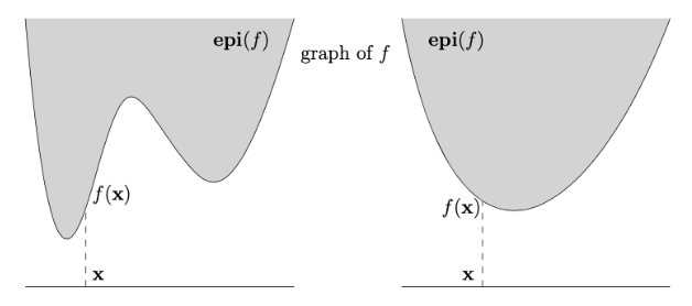
Relationship Between Convex Functions and Sets: Epigraph

Graph of a Function

The graph of a function is defined as:

$$\{(x, f(x)) \mid x \in \text{dom}(f)\}$$

where $\text{dom}(f)$ denotes the domain of $f$.

Epigraph

The epigraph of a function $f: \mathbb{R}^d \to \mathbb{R}$ is:

$$\text{epi}(f) := \{(x, \alpha) \in \mathbb{R}^{d+1} \mid x \in \text{dom}(f), \alpha \geq f(x)\}$$

Note: The epigraph is the set of all points above the function graph, visually the region “above” the function. For convex $f$, the epigraph forms a convex “bowl-shaped” set.

• Key Property:

  $f$ is convex $\iff$ $\text{epi}(f)$ is convex

  Note: This links function convexity to set convexity, simplifying analysis by leveraging convex set properties (e.g., segments lie within the set).

Proof: $f$ convex $\iff$ $\text{epi}(f)$ convex

⇒ (Sufficiency): Assume $f$ convex. Take any $(x,t), (y,s) \in \text{epi}(f)$. Prove segment $\lambda(x,t) + (1-\lambda)(y,s)$ is in $\text{epi}(f)$, i.e.:

$$f(\lambda x + (1-\lambda)y) \leq \lambda t + (1-\lambda)s$$

By convexity of $f$ ($f(\lambda x + (1-\lambda)y) \leq \lambda f(x) + (1-\lambda)f(y)$) and since $(x,t), (y,s) \in \text{epi}(f)$ imply $t \geq f(x)$, $s \geq f(y)$, the inequality holds. Thus $\text{epi}(f)$ is convex.

⇐ (Necessity): Assume $\text{epi}(f)$ convex. Take points $(x,f(x)), (y,f(y)) \in \text{epi}(f)$. Since $\text{epi}(f)$ convex, segment $\lambda(x,f(x)) + (1-\lambda)(y,f(y))$ is in $\text{epi}(f)$, i.e.:

$$(\lambda x + (1-\lambda)y, \lambda f(x) + (1-\lambda)f(y)) \in \text{epi}(f)$$

By epigraph definition, $\lambda f(x) + (1-\lambda)f(y) \geq f(\lambda x + (1-\lambda)y)$, equivalent to $f(\lambda x + (1-\lambda)y) \leq \lambda f(x) + (1-\lambda)f(y)$. Thus $f$ is convex.

Note: Proof uses the epigraph inequality $\alpha \geq f(x)$ to convert set convexity to function convexity. Part 1 derives set convexity from function convexity, Part 2 reverses.

Jensen’s Inequality

Lemma 1 (Jensen’s Inequality)
Let $f$ be convex, $x_1, \dots, x_m \in \text{dom}(f)$, $\lambda_1, \dots, \lambda_m \in \mathbb{R}_+$ with $\sum_{i=1}^m \lambda_i = 1$. Then:

$$f\left( \sum_{i=1}^m \lambda_i x_i \right) \leq \sum_{i=1}^m \lambda_i f(x_i)$$

Note:

• For $m=2$, this reduces to convex function definition.
• General case proven by induction (exercise). Core idea: decompose convex combination recursively.

---

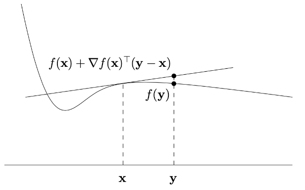
Geometric Properties of Differentiable Functions

For differentiable $f$, the affine function:

$$f(x) + \nabla f(x)^\top (y - x)$$

describes the tangent hyperplane to $f$ at $(x, f(x))$.

Geometric Interpretation:

• $\nabla f(x)$ is the gradient (multidimensional derivative) at $x$.
• This tangent hyperplane touches $f$’s surface at $x$ and locally approximates $f$.
• If $f$ convex, the tangent hyperplane lies below the entire function graph.

---

Convexity Criteria

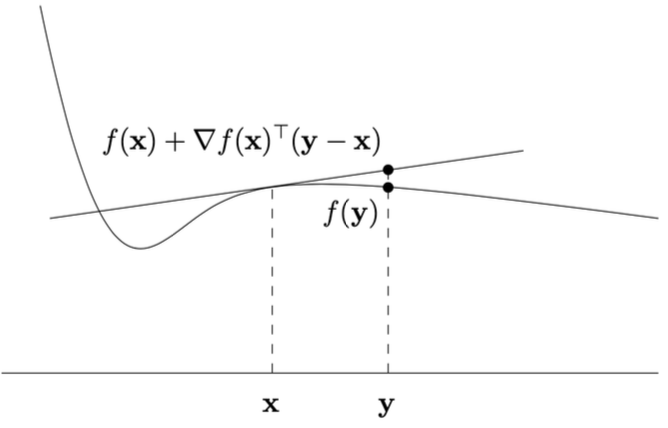
First-Order Convexity Condition

Lemma 2
Assume $\text{dom}(f)$ open and $f$ differentiable (gradient $\nabla f(x) := \left( \frac{\partial f}{\partial x_1}(x), \dots, \frac{\partial f}{\partial x_d}(x) \right)$ exists everywhere). Then $f$ convex iff:

1. $\text{dom}(f)$ convex;

2. For all $x, y \in \text{dom}(f)$:

$$f(y) \geq f(x) + \nabla f(x)^\top (y - x)$$

Geometric Interpretation:

• Inequality means convex function graph lies above its tangent hyperplane at any point (“bowl-shaped”).
• Gradient $\nabla f(x)$ is the steepest ascent direction, $-\nabla f(x)$ the steepest descent.

---

Second-Order Convexity Condition

Assume $\text{dom}(f)$ open and $f$ twice differentiable (Hessian $\nabla^2 f(x)$ symmetric and exists everywhere). Then $f$ convex iff:

1. $\text{dom}(f)$ convex;

2. For all $x \in \text{dom}(f)$, Hessian is positive semi-definite ($\nabla^2 f(x) \succeq 0$), i.e.:

$$\forall z \in \mathbb{R}^d, \quad z^\top \nabla^2 f(x) z \geq 0$$

Key Concepts:

• Hessian Matrix: Symmetric matrix of second partial derivatives, describing local curvature:

$$\nabla^2 f(x) = \begin{pmatrix} \frac{\partial^2 f}{\partial x_1^2} & \cdots & \frac{\partial^2 f}{\partial x_1 \partial x_d} \\ \vdots & \ddots & \vdots \\ \frac{\partial^2 f}{\partial x_d \partial x_1} & \cdots & \frac{\partial^2 f}{\partial x_d^2} \end{pmatrix}$$

• Positive Semi-Definiteness ($\succeq 0$): Non-negative eigenvalues, indicating “upward curvature” in all directions (e.g., Hessian of $x^2$ is 2).

Example

Hessian of $f(x_1, x_2) = x_1^2 + x_2^2$:

$$\nabla^2 f(x) = \begin{pmatrix} 2 & 0 \\ 0 & 2 \end{pmatrix} \succeq 0$$

Note: This matrix is positive definite (eigenvalues 2 > 0), so $f$ is strictly convex (rotational paraboloid).

---

Properties of Convex Functions

Convexity-Preserving Operations

Lemma 4
(i) Let $f_1, \dots, f_m$ be convex, $\lambda_1, \dots, \lambda_m \in \mathbb{R}_+$. Then $f := \sum_{i=1}^m \lambda_i f_i$ is convex on $\text{dom}(f) := \bigcap_{i=1}^m \text{dom}(f_i)$.

Note: Non-negative linear combinations of convex functions remain convex (domain is intersection).

(ii) Let $f$ convex ($\text{dom}(f) \subseteq \mathbb{R}^d$), $g(x) = Ax + b$ affine ($A \in \mathbb{R}^{d \times m}, b \in \mathbb{R}^d$). Then $f \circ g$ (i.e., $x \mapsto f(Ax + b)$) is convex on $\text{dom}(f \circ g) := \{x \in \mathbb{R}^m : Ax + b \in \text{dom}(f)\}$.

Note: Composition with affine mapping preserves convexity (e.g., $f(2x+1)$ convex).

---

Local Minimum is Global Minimum

Definition: $x$ is a local minimum of $f$ if $\exists \varepsilon > 0$ such that $f(x) \leq f(y)$ for all $y \in \text{dom}(f)$ with $\|y - x\| \leq \varepsilon$.

Lemma 5: Local minimum $x^*$ of convex $f$ is a global minimum (i.e., $f(x^*) \leq f(y), \forall y \in \text{dom}(f)$).
Proof:
Assume $\exists y$ with $f(y) < f(x^*)$. Construct $y' = \lambda x^* + (1-\lambda)y$ ($\lambda \in (0,1)$). By convexity:

$$f(y') \leq \lambda f(x^*) + (1-\lambda)f(y) < f(x^*).$$

As $\lambda \to 1$, $\|y' - x^*\| \to 0$, contradicting $x^*$ being local minimum.

---

Critical Point is Global Minimum

Lemma 6: If $f$ differentiable and convex on open convex set $\text{dom}(f)$, and $\nabla f(x) = 0$ (critical point), then $x$ is global minimum.
Proof:
By first-order condition (Lemma 2), for any $y$:

$$f(y) \geq f(x) + \underbrace{\nabla f(x)^\top (y - x)}_{=0} = f(x).$$

Geometric Interpretation: Zero gradient implies horizontal tangent hyperplane and global minimum.

---

Strictly Convex Functions

Definition: $f$ is strictly convex if:

1. $\text{dom}(f)$ convex;

2. For all $x \neq y$ and $\lambda \in (0,1)$:

$$f(\lambda x + (1-\lambda)y) < \lambda f(x) + (1-\lambda)f(y).$$

Examples:

• $x^2$ strictly convex (left);
• Linear functions convex but not strictly convex (right).

Lemma 7: Strictly convex functions have at most one global minimum.

---

Constrained Minimization

Definition: Let $f$ convex, $X \subseteq \text{dom}(f)$ convex. $x \in X$ minimizes $f$ on $X$ if $f(x) \leq f(y), \forall y \in X$.

Lemma 8: If $f$ differentiable on open convex $\text{dom}(f)$, $X \subseteq \text{dom}(f)$ convex, then $x^* \in X$ is minimum iff:

$$\nabla f(x^*)^\top (x - x^*) \geq 0, \quad \forall x \in X.$$

Geometric Interpretation: At $x^*$, gradient forms angle $\leq 90^\circ$ with feasible directions (no descent direction).

---

Existence of Minimum

$\alpha$-Sublevel Set: $f_{\leq \alpha} := \{x \in \mathbb{R}^d : f(x) \leq \alpha\}$.

Note: Even if $f$ bounded below (e.g., $f(x)=e^x$), minimum may not exist (requires sublevel sets compact).

---

Convex Optimization Problems

Form:

$$\min_{x \in D} f(x),$$

with $f$ convex, $D \subseteq \text{dom}(f)$ convex (e.g., $D = \mathbb{R}^d$).
Key Properties:

• Local minimum is global minimum.

• Algorithms (coordinate descent, gradient descent, SGD, etc.) provably converge to global optimum.

Convergence Rate Example: Gradient descent converges at $O(1/t)$ rate:

$$f(x_t) - f(x^*) \leq \frac{c}{t},$$

where $x^*$ is optimum, $c$ constant (depends on initialization and function properties).