SDSC6015 Course 2-Gradient Descent Method and Subgradient Method

#sdsc6015

English / Chinese

Review - Convex Functions and Convex Optimization

Review

Definition of Convex Functions

Review

A function $f: \mathbb{R}^d \to \mathbb{R}$ is convex if and only if:

1. Its domain $\text{dom}(f)$ is a convex set;

2. For all $\mathbf{x}, \mathbf{y} \in \text{dom}(f)$ and $\lambda \in [0,1]$, it satisfies:

   $$f(\lambda \mathbf{x} + (1-\lambda)\mathbf{y}) \leq \lambda f(\mathbf{x}) + (1-\lambda)f(\mathbf{y})$$

Geometric Interpretation: The line segment between any two points on the function’s graph lies above the graph.

---

First-Order Convexity Criterion

Review

If $f$ is differentiable, convexity is equivalent to:

$$f(\mathbf{y}) \geq f(\mathbf{x}) + \nabla f(\mathbf{x})^\top (\mathbf{y} - \mathbf{x}), \quad \forall \mathbf{x}, \mathbf{y} \in \text{dom}(f)$$

Geometric Interpretation: The function graph always lies above its tangent hyperplane.

---

Differentiable Functions

Review

• Definition: $f$ is differentiable at $\mathbf{x}_0$ if there exists a gradient $\nabla f(\mathbf{x}_0)$ such that:

  $$f(\mathbf{x}_0 + \mathbf{h}) \approx f(\mathbf{x}_0) + \nabla f(\mathbf{x}_0)^\top \mathbf{h}$$

  where $\mathbf{h}$ is an infinitesimal perturbation.

• Globally Differentiable: If differentiable at every point in the domain, $f$ is called differentiable, and its graph has non-vertical tangent hyperplanes at all points.

---

Convex Optimization Problems

Review

Formulation:

$$\min_{\mathbf{x} \in \mathbb{R}^d} f(\mathbf{x})$$

where $f$ is a convex differentiable function, and $\mathbb{R}^d$ is a convex set. The global minimum point is denoted $\mathbf{x}^* = \arg\min f(\mathbf{x})$ (may not be unique).

---

Gradient Descent Method

Core Idea

Update parameters using the negative gradient direction (gradient $\nabla f(\mathbf{x})$ points in the direction of fastest function increase):

$$\mathbf{x}_{k+1} = \mathbf{x}_k - \eta_k \nabla f(\mathbf{x}_k)$$

where:

• $\mathbf{x}_k$: Current parameter vector at iteration $k$

• $\eta_k$: Step size (learning rate), controlling update magnitude ($\eta_k > 0$)

• $\nabla f(\mathbf{x}_k)$: Gradient of $f$ at $\mathbf{x}_k$

• $\mathbf{x}_{k+1}$: Updated parameter vector

Key Notes:

1. Gradient Direction: Negative gradient $-\nabla f(\mathbf{x}_k)$ points in the direction of fastest function decrease;
2. Step Size Selection:
   • Fixed step size (e.g., $\eta_k = 0.1$) must satisfy convergence conditions;
   • Adaptive step size (e.g., $\eta_k = \frac{1}{\sqrt{k}}$) improves convergence;
3. Geometric Meaning: Each iteration moves linearly along the gradient direction by distance $\eta_k \|\nabla f(\mathbf{x}_k)\|$.

---

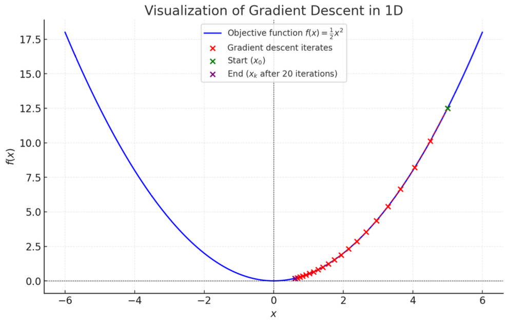
Gradient Descent Example: Quadratic Function Optimization

Consider the convex function $f(x) = \frac{1}{2} x^2$:

• Minimum Point: $x^* = 0$ (minimum value $f(0)=0$)

• Gradient Calculation:

  $$\nabla f(x) = \frac{d}{dx} \left( \frac{1}{2} x^2 \right) = x$$

Gradient Descent Update Rule

Iteration formula with fixed step size $\eta$:

$$x_{t+1} = x_t - \eta \nabla f(x_t) = x_t - \eta x_t = x_t (1 - \eta)$$

• $x_t$: Parameter value at iteration $t$

• $\eta$: Step size (learning rate)

Closed-Form Iteration Sequence

After $k$ iterations:

$$x_k = x_0 (1 - \eta)^k$$

Derivation:
Recursive expansion:

$$x_k = x_{k-1} (1 - \eta) = x_{k-2} (1 - \eta)^2 = \cdots = x_0 (1 - \eta)^k$$

Convergence Analysis

When $0 < \eta < 1$:

$$\lim_{k \to \infty} x_k = \lim_{k \to \infty} x_0 (1 - \eta)^k = 0$$

Explanation:
Since $|1 - \eta| < 1$, the sequence $(1 - \eta)^k$ decays exponentially to 0, so iterates converge to $x^* = 0$.

---

Convergence Behavior with Specific Parameters

• Step Size: $\eta = 0.1$

• Initial Point: $x_0 = 5$

• Iteration Sequence:

  $$x_k = 5 \times (0.9)^k$$

• Convergence Process:

  • $k=0$: $x_0 = 5$
  • $k=1$: $x_1 = 5 \times 0.9 = 4.5$
  • $k=10$: $x_{10} = 5 \times (0.9)^{10} \approx 1.74$
  • $k=50$: $x_{50} = 5 \times (0.9)^{50} \approx 0.034$ (close to minimum)

Conclusion:
This example verifies global convergence of gradient descent on convex functions. Step size $\eta=0.1$ satisfies $0<\eta<1$, ensuring monotonic convergence to $x^*=0$.

---

Vanilla Analysis of Gradient Descent

Goal: Bound the error $f(\mathbf{x}_t) - f(\mathbf{x}^*)$

Define gradient $\mathbf{g}_t := \nabla f(\mathbf{x}_t)$. From update rule $\mathbf{x}_{t+1} = \mathbf{x}_t - \eta \mathbf{g}_t$:

$$\mathbf{g}_t = \frac{\mathbf{x}_t - \mathbf{x}_{t+1}}{\eta}$$

Key Equality Derivation

1. Construct Inner Product Term:

   $$\mathbf{g}_t^\top (\mathbf{x}_t - \mathbf{x}^*) = \frac{1}{\eta} (\mathbf{x}_t - \mathbf{x}_{t+1})^\top (\mathbf{x}_t - \mathbf{x}^*)$$

2. Apply Vector Identity ($2\mathbf{v}^\top\mathbf{w} = \|\mathbf{v}\|^2 + \|\mathbf{w}\|^2 - \|\mathbf{v} - \mathbf{w}\|^2$):

   $$\begin{aligned} \mathbf{g}_t^\top (\mathbf{x}_t - \mathbf{x}^*) &= \frac{1}{2\eta} \left( \|\mathbf{x}_t - \mathbf{x}_{t+1}\|^2 + \|\mathbf{x}_t - \mathbf{x}^*\|^2 - \|\mathbf{x}_{t+1} - \mathbf{x}^*\|^2 \right) \\ &= \frac{\eta}{2} \|\mathbf{g}_t\|^2 + \frac{1}{2\eta} \left( \|\mathbf{x}_t - \mathbf{x}^*\|^2 - \|\mathbf{x}_{t+1} - \mathbf{x}^*\|^2 \right) \end{aligned}$$

   Notes:

   • Term $\frac{\eta}{2} \|\mathbf{g}_t\|^2$ controls gradient magnitude;
   • Term $\frac{1}{2\eta} (\|\mathbf{x}_t - \mathbf{x}^*\|^2 - \|\mathbf{x}_{t+1} - \mathbf{x}^*\|^2)$ represents distance change in parameter space.

3. Sum over $T$ Steps:

   $$\sum_{t=0}^{T-1} \mathbf{g}_t^\top (\mathbf{x}_t - \mathbf{x}^*) = \frac{\eta}{2} \sum_{t=0}^{T-1} \|\mathbf{g}_t\|^2 + \frac{1}{2\eta} \left( \|\mathbf{x}_0 - \mathbf{x}^*\|^2 - \|\mathbf{x}_T - \mathbf{x}^*\|^2 \right)$$

Combine with First-Order Convexity Condition

From convexity: $f(\mathbf{x}^*) \geq f(\mathbf{x}_t) + \mathbf{g}_t^\top (\mathbf{x}^* - \mathbf{x}_t)$, yielding per-step error bound:

$$f(\mathbf{x}_t) - f(\mathbf{x}^*) \leq \mathbf{g}_t^\top (\mathbf{x}_t - \mathbf{x}^*)$$

Substitute into summation for cumulative error bound:

$$\sum_{t=0}^{T-1} \left[ f(\mathbf{x}_t) - f(\mathbf{x}^*) \right] \leq \frac{\eta}{2} \sum_{t=0}^{T-1} \|\mathbf{g}_t\|^2 + \frac{1}{2\eta} \left( \|\mathbf{x}_0 - \mathbf{x}^*\|^2 - \|\mathbf{x}_T - \mathbf{x}^*\|^2 \right)$$

Key Conclusions:

1. Cumulative error is controlled by gradient norm sum $\sum \|\mathbf{g}_t\|^2$ and initial distance $\|\mathbf{x}_0 - \mathbf{x}^*\|^2$;
2. Step Size $\eta$ Trade-off:
   • Too large: Gradient term $\frac{\eta}{2} \sum \|\mathbf{g}_t\|^2$ dominates, may diverge;
   • Too small: Distance term $\frac{1}{2\eta} \|\mathbf{x}_0 - \mathbf{x}^*\|^2$ dominates, slow convergence.

---

Convergence Analysis for Lipschitz Convex Functions

Assume all gradients of f have bounded norm.

• Equivalent to $f$ being Lipschitz (see notes)

• Excludes many interesting functions (e.g., $f(x) = x^2$)

Equivalence Proof

Let $f: \mathbb{R}^d \to \mathbb{R}$ be convex. The following are equivalent:

1. Bounded Gradient: $\exists M > 0$ such that $\|\nabla f(x)\| \leq M, \ \forall x$.

2. Lipschitz Continuity: $\exists L > 0$ such that $\|f(y) - f(x)\| \leq L \|y - x\|, \ \forall x, y$.

---

Proof Outline

(⇒) Bounded Gradient ⇒ Lipschitz Continuity

Assume $\|\nabla f(x)\| \leq M$. By fundamental theorem of calculus:

$$f(y) - f(x) = \int_0^1 \nabla f(x + t(y-x))^\top (y-x) \, dt$$

Take norms and apply Cauchy-Schwarz:

$$\|f(y) - f(x)\| \leq \int_0^1 \|\nabla f(x + t(y-x))\| \cdot \|y - x\| \, dt$$

Substitute bounded gradient condition:

$$\|f(y) - f(x)\| \leq \int_0^1 M \|y - x\| \, dt = M \|y - x\|$$

Thus $f$ is $M$-Lipschitz.

Explanation: Bounded gradient norm controls function value change rate.

---

(⇐) Lipschitz Continuity ⇒ Bounded Gradient

Assume $\|f(y) - f(x)\| \leq L \|y - x\|$ and $f$ convex. Need $\|\nabla f(x)\| \leq L$.

• If $\nabla f(x) = 0$: Trivial.

• Otherwise: Set $y = x + \nabla f(x)$.
  By first-order convexity condition:

  $$f(y) \geq f(x) + \nabla f(x)^\top (y - x)$$

  Substitute $y - x = \nabla f(x)$:

  $$f(y) - f(x) \geq \nabla f(x)^\top \nabla f(x) = \|\nabla f(x)\|^2 \quad (*)$$

  By Lipschitz continuity:

  $$f(y) - f(x) \leq L \|y - x\| = L \|\nabla f(x)\| \quad (**)$$

  Combine $(*)$ and $(**)$:

  $$\|\nabla f(x)\|^2 \leq L \|\nabla f(x)\|$$

  Thus $\|\nabla f(x)\| \leq L$.

Explanation: Lipschitz continuity restricts linear growth of function values, forcing bounded gradient norm.

---

Key Formula Notes

1. Fundamental Theorem Application:

   $$f(y) - f(x) = \int_0^1 \nabla f(x + t(y-x))^\top (y-x) \, dt$$

   • Meaning: Expresses function difference as path integral of gradient.

2. Cauchy-Schwarz Inequality:

   $$\left| \nabla f(z)^\top (y-x) \right| \leq \|\nabla f(z)\| \cdot \|y - x\|$$

   • Role: Converts inner product to norm product for integral bounding.

3. First-Order Convexity Condition:

   $$f(y) \geq f(x) + \nabla f(x)^\top (y - x)$$

   • Role: Establishes one-way relationship between gradient and function value change.

---

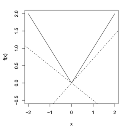
Appendix: P47 Example
For $f(x) = |x|$:

• At $x > 0$, $g_k = 1$, gradient descent may overshoot $x^* = 0$.
• At $x = 0$, subgradient $g_k \in [-1, 1]$ causes oscillation.
  Non-smooth functions require specialized methods (e.g., subgradient method).

---

Theorem Setup

Let $f: \mathbb{R}^d \to \mathbb{R}$ be convex differentiable with:

1. $\|\mathbf{x}_0 - \mathbf{x}^*\| \leq R$ (bounded initial distance)

2. $\|\nabla f(\mathbf{x})\| \leq B,\ \forall \mathbf{x}$ (bounded gradient norm, equivalent to $B$-Lipschitz $f$)

Convergence Proof

1. Base Inequality (from Vanilla Analysis):

   $$\sum_{t=0}^{T-1} [f(\mathbf{x}_t) - f(\mathbf{x}^*)] \leq \frac{\eta}{2} \sum_{t=0}^{T-1} \|\mathbf{g}_t\|^2 + \frac{1}{2\eta} \|\mathbf{x}_0 - \mathbf{x}^*\|^2$$

2. Substitute Bounded Conditions:

   $$\sum_{t=0}^{T-1} [f(\mathbf{x}_t) - f(\mathbf{x}^*)] \leq \frac{\eta}{2} B^2 T + \frac{R^2}{2\eta}$$

3. Optimize Step Size $\eta$:
   Define auxiliary function:

   $$h(\eta) = \frac{\eta B^2 T}{2} + \frac{R^2}{2\eta}$$

   • Optimal step size via derivative:

     $$h'(\eta) = \frac{B^2 T}{2} - \frac{R^2}{2\eta^2} = 0 \ \Rightarrow \ \eta^* = \frac{R}{B\sqrt{T}}$$

   • Substitute for minimal bound:

     $$h(\eta^*) = \frac{R}{B\sqrt{T}} \cdot \frac{B^2 T}{2} + \frac{R^2}{2 \cdot \frac{R}{B\sqrt{T}}} = RB\sqrt{T}$$

4. Average Error Bound:

   $$\frac{1}{T} \sum_{t=0}^{T-1} [f(\mathbf{x}_t) - f(\mathbf{x}^*)] \leq \frac{RB}{\sqrt{T}}$$

Convergence Rate and Iteration Count

• Iterations for $\varepsilon$-accuracy:

  $$T \geq \frac{R^2 B^2}{\varepsilon^2} \quad \Rightarrow \quad \frac{RB}{\sqrt{T}} \leq \varepsilon$$

• Advantages:

  1. Dimension Independence: Rate independent of dimension $d$
  2. Robustness: Holds for both average iterate $\frac{1}{T}\sum f(\mathbf{x}_t)$ and best iterate $\min_t f(\mathbf{x}_t)$

Note: Lipschitz condition excludes functions with unbounded gradients (e.g., $f(x)=x^2$), which require smoothness analysis.

Practical Advice (Unknown $R$, $B$)

1. Fixed Small Step Size: Start with $\eta = 0.01$

2. Dynamic Adjustment:

   • Oscillation/divergence → decrease $\eta$
   • Or use decaying step size $\eta_t = \frac{\eta_0}{\sqrt{t+1}}$

3. Adaptive Methods: Use adaptive optimizers like Adam

---

Smooth Functions

Definition

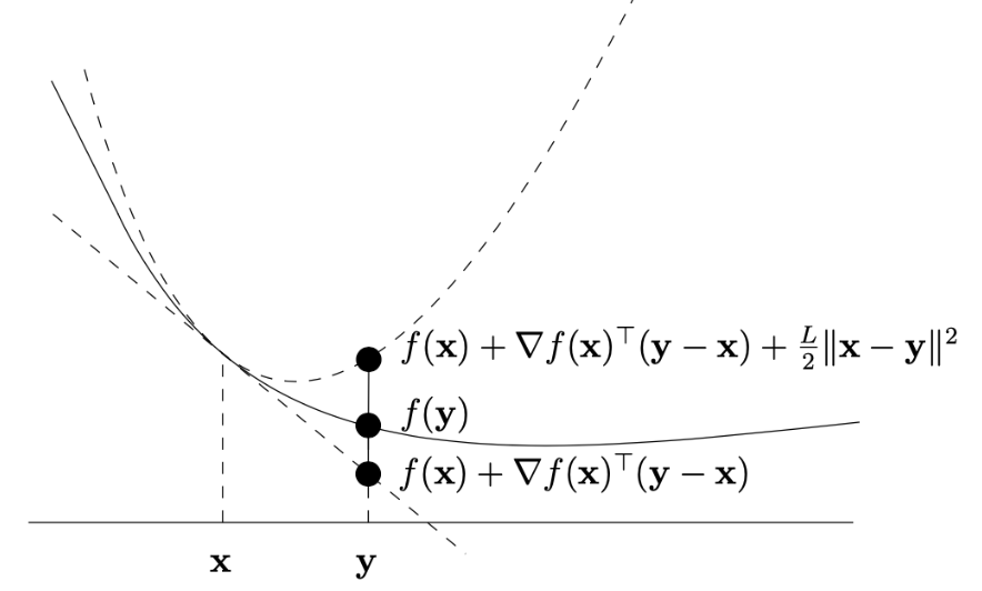
A differentiable function $f : \text{dom}(f) \to \mathbb{R}$ is smooth with parameter $L > 0$ on subset $X \subseteq \text{dom}(f)$ if for all $x, y \in X$:

$$f(y) \leq f(x) + \nabla f(x)^\top (y - x) + \frac{L}{2} \|x - y\|^2$$

Intuition:

• The function “does not bend too much,” its growth is bounded by a quadratic function (like a paraboloid).
• $L$ quantifies the maximum rate of gradient change (faster gradient changes → larger $L$).

---

Geometric Interpretation

Smoothness implies: Near any point $x$, $f$ is upper-bounded by a quadratic function (paraboloid-shaped graph).

Example:
Quadratic functions (e.g., $f(x) = x^2$) are smooth.

---

Operations Preserving Smoothness

The following operations preserve smoothness under specified conditions:

Lemma 1
(i) Let $f_1, \dots, f_m$ be smooth with parameters $L_1, \dots, L_m$, weights $\lambda_1, \dots, \lambda_m \in \mathbb{R}^+$. Then $f := \sum_{i=1}^m \lambda_i f_i$ is smooth with parameter $\sum_{i=1}^m \lambda_i L_i$.
(ii) Let $f$ be smooth (parameter $L$), $g: \mathbb{R}^m \to \mathbb{R}^d$ affine (i.e., $g(x) = Ax + b$, $A \in \mathbb{R}^{d \times m}$, $b \in \mathbb{R}^d$). Then $f \circ g$ ($x \mapsto f(Ax + b)$) is smooth with parameter $L \|A\|_2$.

Here $\|A\|_2$ is the spectral norm of $A$ (largest singular value).

---

Convex vs. Smooth Functions: Properties and Optimization

Basic Concept Comparison

Property	Mathematical Definition	Geometric Meaning	Optimization Implication
Convexity	$f(\lambda x + (1-\lambda)y) \leq \lambda f(x) + (1-\lambda)f(y)$	Graph below chords	Guarantees global optimality
Lipschitz Continuity	$|\nabla f(x)| \leq B$	Bounded gradient, controlled change rate	Controls gradient descent stability
Smoothness	$|\nabla f(x) - \nabla f(y)| \leq L|x-y|$	Gentle gradient changes, bounded curvature	Enables faster convergence rates

Key Equivalence

Lemma 2: Equivalent Characterizations of Smoothness

For convex differentiable $f: \mathbb{R}^d \to \mathbb{R}$, the following are equivalent:

1. $f$ is $L$-smooth: $f(y) \leq f(x) + \nabla f(x)^\top(y-x) + \frac{L}{2}\|x-y\|^2$

2. Gradient is $L$-Lipschitz: $\|\nabla f(x) - \nabla f(y)\| \leq L\|x-y\|$

Significance: Establishes equivalence between function smoothness and gradient Lipschitz continuity.

Gradient Descent Analysis for Smooth Functions

Lemma 3: Sufficient Decrease

For $L$-smooth functions, gradient descent with $\eta = \frac{1}{L}$ satisfies:

$$f(x_{t+1}) \leq f(x_t) - \frac{1}{2L} \|\nabla f(x_t)\|^2$$

Proof:

$$\begin{aligned} f(x_{t+1}) &\leq f(x_t) + \nabla f(x_t)^\top(x_{t+1}-x_t) + \frac{L}{2}\|x_{t+1}-x_t\|^2 \\ &= f(x_t) - \frac{1}{L} \|\nabla f(x_t)\|^2 + \frac{1}{2L} \|\nabla f(x_t)\|^2 \\ &= f(x_t) - \frac{1}{2L} \|\nabla f(x_t)\|^2 \end{aligned}$$

Meaning: Each iteration guarantees function value decrease, controlled by gradient norm.

Theorem 2: Convergence Rate

For $L$-smooth convex $f$, gradient descent with $\eta = \frac{1}{L}$ satisfies:

$$f(x_T) - f(x^*) \leq \frac{L \|x_0 - x^*\|^2}{2T}$$

Proof Sketch:

1. Use base analysis inequality

2. Apply sufficient decrease lemma to bound gradient term

3. Obtain final bound via telescoping sum

Practical Applications and Comparisons

Convergence Rate Comparison

Function Type	Convergence Rate	Iteration Complexity ($\varepsilon$-accuracy)
Lipschitz Convex	$O(1/\sqrt{T})$	$O(1/\varepsilon^2)$
Smooth Convex	$O(1/T)$	$O(1/\varepsilon)$

Advantage: Smoothness improves convergence from sublinear to linear, significantly boosting efficiency.

Practical Advice: Unknown $L$

1. Initial Guess: Set $L = \frac{2\varepsilon}{R^2}$ (if correct, one iteration suffices)

2. Verification: Check $f(x_{t+1}) \leq f(x_t) - \frac{1}{2L} \|\nabla f(x_t)\|^2$

3. Doubling Strategy: If condition fails, double $L$ and retry

4. Total Complexity: At most $O\left(\frac{4R^2L}{\varepsilon}\right)$ iterations for $\varepsilon$-accuracy

Practical Impact: Adaptive adjustment enables efficient optimization even without knowing $L$.

---

Subgradient Method

Subgradient Definition

For convex $f: \mathbb{R}^d \to \mathbb{R}$, a subgradient at $\mathbf{x}$ is any vector $\mathbf{g} \in \mathbb{R}^d$ satisfying:

$$f(\mathbf{y}) \geq f(\mathbf{x}) + \mathbf{g}^\top (\mathbf{y} - \mathbf{x}), \quad \forall \mathbf{y}$$

Key Properties:

• Always exists at points in the domain
• If $f$ differentiable at $\mathbf{x}$, subgradient unique and equals $\nabla f(\mathbf{x})$

Subgradient Calculation Examples

Example 1: Absolute Value $f(x) = |x|$

• For $x \neq 0$: Unique subgradient $g = \text{sign}(x)$

• For $x = 0$: Any $g \in [-1, 1]$

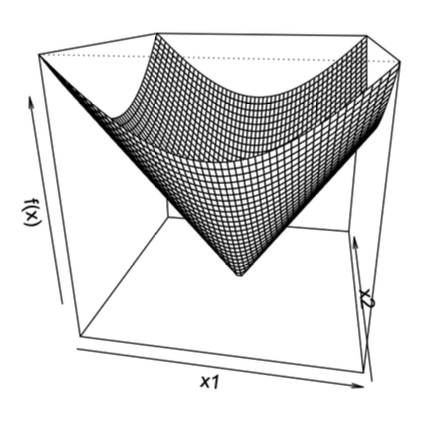
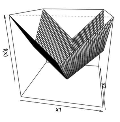
Example 2: L2 Norm $f(\mathbf{x}) = \|\mathbf{x}\|_2$

• For $\mathbf{x} \neq \mathbf{0}$: Unique subgradient $\mathbf{g} = \frac{\mathbf{x}}{\|\mathbf{x}\|_2}$

• For $\mathbf{x} = \mathbf{0}$: Any $\mathbf{g}$ in closed unit ball $\{\mathbf{z} : \|\mathbf{z}\|_2 \leq 1\}$

Example 3: L1 Norm $f(\mathbf{x}) = \|\mathbf{x}\|_1 = \sum_{i=1}^d |x_i|$

• For $x_i \neq 0$: Component $g_i = \text{sign}(x_i)$

• For $x_i = 0$: Component $g_i \in [-1, 1]$

Example 4: Set Indicator Function

For convex set $X \subset \mathbb{R}^d$:

$$1_X(\mathbf{x}) = \begin{cases} 0 & \text{if } \mathbf{x} \in X \\ +\infty & \text{if } \mathbf{x} \notin X \end{cases}$$

Normal Cone

Definition: For convex set $X \subseteq \mathbb{R}^d$ and point $\mathbf{x} \in X$, the normal cone is:

$$\mathcal{N}_X(\mathbf{x}) = \{ \mathbf{g} \in \mathbb{R}^d \mid \mathbf{g}^\top \mathbf{x} \geq \mathbf{g}^\top \mathbf{y},\ \forall \mathbf{y} \in X \}$$

Geometric Interpretation: Contains outward-pointing vectors “supporting” $X$ at $\mathbf{x}$. These vectors form right/obtuse angles with all feasible directions at $\mathbf{x}$.

Subdifferential

Definition: The subdifferential of convex $f: \mathbb{R}^d \to \mathbb{R}$ at $\mathbf{x}$ is the set of all subgradients:

$$\partial f(\mathbf{x}) = \{ \mathbf{g} \in \mathbb{R}^d \mid f(\mathbf{y}) \geq f(\mathbf{x}) + \mathbf{g}^\top (\mathbf{y} - \mathbf{x}),\ \forall \mathbf{y} \in \mathbb{R}^d \}$$

Properties:

• $\partial f(\mathbf{x})$ is closed and convex

• If $f$ differentiable at $\mathbf{x}$, $\partial f(\mathbf{x}) = \{ \nabla f(\mathbf{x}) \}$

• If $\partial f(\mathbf{x})$ is singleton, $f$ differentiable at $\mathbf{x}$ with $\nabla f(\mathbf{x}) = \mathbf{g}$

Optimality Conditions

Unconstrained Optimization

For convex $f: \mathbb{R}^d \to \mathbb{R}$:

$$\mathbf{x}^* \text{ minimizes } f \iff 0 \in \partial f(\mathbf{x}^*)$$

Interpretation: $\mathbf{x}^*$ is minimum iff zero vector is a subgradient.

Constrained Optimization

Consider:

$$\min_{\mathbf{x}} f(\mathbf{x}) \quad \text{s.t.} \quad \mathbf{x} \in X$$

Reformulation: Introduce indicator function $1_X(\mathbf{x})$:

$$\min_{\mathbf{x}} \left\{ f(\mathbf{x}) + 1_X(\mathbf{x}) \right\}$$

Optimality Condition: $\mathbf{x}^* \in X$ is optimal iff:

$$0 \in \partial \left( f(\mathbf{x}^*) + 1_X(\mathbf{x}^*) \right) = \nabla f(\mathbf{x}^*) + \mathcal{N}_X(\mathbf{x}^*)$$

Equivalently:

$$- \nabla f(\mathbf{x}^*) \in \mathcal{N}_X(\mathbf{x}^*)$$

By normal cone definition, this means:

$$\nabla f(\mathbf{x}^*)^\top (\mathbf{y} - \mathbf{x}^*) \geq 0, \quad \forall \mathbf{y} \in X$$

Geometric Interpretation: At optimum $\mathbf{x}^*$, the gradient points opposite to feasible directions.

---

Subgradient Method

Basic Concepts

For a convex function $f : \mathbb{R}^d \to \mathbb{R}$ (not necessarily differentiable), the subgradient method mimics gradient descent but uses a subgradient instead of the gradient:

$$x_{k+1} = x_k - \eta_{k+1} g_k$$

• $x_k$: current point

• $g_k \in \nabla f(x_k)$: any subgradient of $f$ at $x_k$

• $\eta_k > 0$: step size

• $x_{k+1}$: updated next point

⚠️ Note: The subgradient method is not necessarily a descent method. For example, when $f(x) = |x|$, non-smoothness can cause oscillations.

Convergence Theorem

Theorem 3: Assume $f$ is convex and L-Lipschitz (i.e., $|f(x) - f(y)| \leq L \|x - y\|$).

1. Fixed step size $\eta_k = \eta$ (for all $k$):

   $$\lim_{k \to \infty} f(x_{\text{best}}^{(k)}) \leq f^* + \frac{L^2 \eta}{2}$$

2. Diminishing step size (satisfying $\sum_{k=1}^\infty \eta_k^2 < \infty$ and $\sum_{k=1}^\infty \eta_k = \infty$):

   $$\lim_{k \to \infty} f(x_{\text{best}}^{(k)}) \leq f^*$$

Where:

• $f(x_{\text{best}}^{(k)}) = \min_{i=0,\dots,k} f(x_i)$ is the best value up to step $k$
• $f^* = f(x^*)$ is the true minimum value

Key Steps of the Proof

Based on the definition of the subgradient, we can derive the basic inequality:

$$\|x_k - x^*\|^2 \leq \|x_{k-1} - x^*\|^2 - 2\eta_k (f(x_{k-1}) - f^*) + \eta_k^2 \|g_{k-1}\|^2$$

Iterating this inequality and rearranging (let $R = \|x_0 - x^*\|$), we get:

$$0 \leq R^2 - 2 \sum_{i=1}^k \eta_i (f(x_{i-1}) - f^*) + L^2 \sum_{i=1}^k \eta_i^2$$

After introducing $f(x_{\text{best}}^{(k)})$, we obtain the basic inequality:

$$f(x_{\text{best}}^{(k)}) - f^* \leq \frac{R^2 + L^2 \sum_{i=1}^k \eta_i^2}{2 \sum_{i=1}^k \eta_i}$$

The convergence results for different step size strategies can be derived from this.

Convergence Rate with Fixed Step Size

If the step size is fixed as $\eta$, then:

$$f(x_{\text{best}}^{(k)}) - f^* \leq \frac{R^2}{2k\eta} + \frac{L^2 \eta}{2}$$

To achieve accuracy $f(x_{\text{best}}^{(k)}) - f^* \leq \varepsilon$, set each term $\leq \varepsilon/2$, and solve:

• Optimal step size: $\eta = \frac{\varepsilon}{L^2}$

• Required number of iterations: $k = \frac{R^2 L^2}{\varepsilon^2}$

Therefore, the convergence rate of the subgradient method is $O\left(\frac{1}{\varepsilon^2}\right)$.

📉 Comparison: The convergence rate of gradient descent for smooth convex functions is $O\left(\frac{1}{\varepsilon}\right)$, indicating that the subgradient method converges slower.

Summary of Algorithm Convergence

Function Properties	Algorithm	Convergence Bound	Number of Iterations
Convex, L-Lipschitz	Subgradient	$f(x_{\text{best}}^{(T)}) - f^* \leq \frac{LR}{\sqrt{T}}$	$O\left(\frac{R^2 L^2}{\varepsilon^2}\right)$
Convex, L-Smooth	Gradient Descent	$f(x_{\text{best}}^{(T)}) - f^* \leq \frac{R^2 L}{2T}$	$O\left(\frac{R^2 L}{\varepsilon}\right)$
Convex, L-Lipschitz	Gradient Descent	$f(x_{\text{best}}^{(T)}) - f^* \leq \frac{RL}{\sqrt{T}}$	$O\left(\frac{R^2 L^2}{\varepsilon^2}\right)$

Where:

• $T$: time horizon/number of iterations
• $R = \|x_0 - x^*\|$: distance from initial point to optimum
• $x_{\text{best}}^{(T)} = \arg\min_{i=0,1,\dots,T} f(x_i)$: best point among the first $T$ iterations

---

Summary

Expand

Convex Function Definition

$f: \mathbb{R}^d \to \mathbb{R}$ is convex iff:

1. $\text{dom}(f)$ convex;

2. $\forall \mathbf{x}, \mathbf{y} \in \text{dom}(f), \lambda \in [0,1]$:

   $$f(\lambda \mathbf{x} + (1-\lambda)\mathbf{y}) \leq \lambda f(\mathbf{x}) + (1-\lambda)f(\mathbf{y})$$

Geometry: Line segment between graph points lies above graph.

---

First-Order Convexity

If $f$ differentiable, convexity ≡:

$$f(\mathbf{y}) \geq f(\mathbf{x}) + \nabla f(\mathbf{x})^\top (\mathbf{y} - \mathbf{x})$$

Geometry: Graph above tangent hyperplane.

---

Differentiable Functions

• Definition: $f$ differentiable at $\mathbf{x}_0$ if $\exists \nabla f(\mathbf{x}_0)$:

  $$f(\mathbf{x}_0 + \mathbf{h}) \approx f(\mathbf{x}_0) + \nabla f(\mathbf{x}_0)^\top \mathbf{h}$$

• Global Differentiability: Differentiable everywhere → non-vertical tangents everywhere.

---

Convex Optimization

Formulation:

$$\min_{\mathbf{x} \in \mathbb{R}^d} f(\mathbf{x})$$

$f$ convex differentiable, $\mathbb{R}^d$ convex. Minimum $\mathbf{x}^* = \arg\min f(\mathbf{x})$ (may not be unique).

---

Gradient Descent

Core Idea

Update with negative gradient:

$$\mathbf{x}_{k+1} = \mathbf{x}_k - \eta_k \nabla f(\mathbf{x}_k)$$

• $\eta_k$: Step size

• $\mathbf{x}_k$: Current parameters

Convergence Analysis

Lipschitz Convex Functions (Bounded Gradient)

Assumptions: $\|\nabla f(\mathbf{x})\| \leq B$, $\|\mathbf{x}_0 - \mathbf{x}^*\| \leq R$
Step Size: $\eta = \frac{R}{B\sqrt{T}}$
Convergence Rate:

$$\frac{1}{T} \sum_{t=0}^{T-1} [f(\mathbf{x}_t) - f(\mathbf{x}^*)] \leq \frac{RB}{\sqrt{T}}$$

Advantage: Dimension-independent.
Practice: Unknown $B, R$ → try small $\eta$ (e.g., 0.01) or adaptive methods.

Smooth Convex Functions (Lipschitz Gradient)

Definition: $f$ is $L$-smooth if:

$$f(\mathbf{y}) \leq f(\mathbf{x}) + \nabla f(\mathbf{x})^\top (\mathbf{y}-\mathbf{x}) + \frac{L}{2} \|\mathbf{x}-\mathbf{y}\|^2$$

≡ $\|\nabla f(\mathbf{x}) - \nabla f(\mathbf{y})\| \leq L \|\mathbf{x}-\mathbf{y}\|$.
Step Size: $\eta = \frac{1}{L}$
Convergence Rate:

$$f(\mathbf{x}_T) - f(\mathbf{x}^*) \leq \frac{L \|\mathbf{x}_0 - \mathbf{x}^*\|^2}{2T}$$

Comparison: $O(1/\varepsilon)$ for smooth vs. $O(1/\varepsilon^2)$ for Lipschitz.
Practice: Unknown $L$ → doubling strategy with verification of $f(\mathbf{x}_{t+1}) \leq f(\mathbf{x}_t) - \frac{1}{2L} \|\nabla f(\mathbf{x}_t)\|^2$.

---

Subgradient Method

Subgradient Definition

For convex $f$, $g \in \partial f(\mathbf{x})$ satisfies:

$$f(\mathbf{y}) \geq f(\mathbf{x}) + g^\top (\mathbf{y} - \mathbf{x}), \quad \forall \mathbf{y}$$

Key Properties:

• $\partial f(\mathbf{x}) = \{\nabla f(\mathbf{x})\}$ if differentiable;
• Optimality: $\mathbf{x}^*$ minimum iff $0 \in \partial f(\mathbf{x}^*)$.

Update Rule

$$\mathbf{x}_{k+1} = \mathbf{x}_k - \eta_k g_k, \quad g_k \in \partial f(\mathbf{x}_k)$$

Note: Not a descent method (e.g., oscillates for $f(x)=|x|$).

Convergence

Assumptions: $f$ convex $L$-Lipschitz

• Fixed $\eta$: Limiting error $\leq f^* + L^2\eta/2$

• Diminishing $\eta$ ($\sum \eta_k = \infty$, $\sum \eta_k^2 < \infty$): Asymptotic convergence to $f^*$
  Convergence Rate:

$$f(\mathbf{x}_{\text{best}}^{(k)}) - f^* \leq \frac{R^2 + L^2 \sum_{i=1}^k \eta_i^2}{2 \sum_{i=1}^k \eta_i}$$

where $R = \|\mathbf{x}_0 - \mathbf{x}^*\|$, $f_{\text{best}}^{(k)} = \min_{i=0,\dots,k} f(\mathbf{x}_i)$.