SDSC6015 Course 3-Faster Gradient Descent and Subgradient Descent

#sdsc6015

English / 中文

Review

Click to expand

Convex Optimization Problems

The general form of a convex optimization problem is:

$$\min_{x \in \mathbb{R}^d} f(x)$$

where $f$ is a convex function, $\mathbb{R}^d$ is a convex set, and $x^*$ is its minimizer:

$$x^* = \arg\min_{x \in \mathbb{R}^d} f(x)$$

The update rule for Gradient Descent (GD) is:

$$x_{k+1} = x_k - \eta_{k+1} \nabla f(x_k)$$

• $x_k$: current parameter point

• $\eta_k > 0$: step size (learning rate)

• $x_{k+1}$: updated parameter point

---

Smooth Functions

Definition:

A function $f: \text{dom}(f) \to \mathbb{R}$ is differentiable and there exists $L > 0$ such that for all $x, y \in X \subseteq \text{dom}(f)$:

$$f(y) \leq f(x) + \nabla f(x)^\top (y - x) + \frac{L}{2} \|x - y\|^2$$

Then $f$ is called $L$-smooth.

💡 Smoothness means the gradient of the function does not change too quickly, with an upper bound controlled by $L$.

---

Subgradient

Definition:

For a convex function $f: \mathbb{R}^d \to \mathbb{R}$, a subgradient $g$ at point $x$ satisfies:

$$f(y) \geq f(x) + g^\top (y - x), \quad \forall y$$

The set of all subgradients is called the subdifferential:

$$\partial f(x) = \{ g \in \mathbb{R}^d \mid g \text{ is a subgradient of } f \text{ at } x \}$$

🔍 For differentiable convex functions, the subdifferential is the gradient; for non-differentiable functions (e.g., $|x|$), the subgradient may not be unique.

Subgradient Method:

The update rule is:

$$x_{k+1} = x_k - \eta_{k+1} g_k, \quad g_k \in \partial f(x_k)$$

• Note: The subgradient method is not necessarily a descent method (e.g., $f(x) = |x|$ may cause oscillation).

---

Convergence Performance Comparison Table

Function Properties	Algorithm	Convergence Bound	Iterations (to achieve error $\varepsilon$)
Convex, $L$-Lipschitz	GD	$f(x_{\text{best}}^{(T)}) - f(x^*) \leq \frac{RL}{\sqrt{T}}$	$\mathcal{O}\left( \frac{R^2 L^2}{\varepsilon^2} \right)$
Convex, $L$-Smooth	GD	$f(x_{\text{best}}^{(T)}) - f(x^*) \leq \frac{R^2 L}{2T}$	$\mathcal{O}\left( \frac{R^2 L}{2\varepsilon} \right)$
$\mu$-SC, $L$-Smooth	GD	$f(x_{\text{best}}^{(T)}) - f(x^*) \leq \frac{L}{2} \left(1 - \frac{\mu}{L}\right)^T R^2$	$\mathcal{O}\left( \frac{L}{\mu} \ln \frac{R^2 L}{2\varepsilon} \right)$
Convex, $L$-Lipschitz	Subgradient	$f(x_{\text{best}}^{(T)}) - f(x^*) \leq \frac{LR}{\sqrt{T}}$	$\mathcal{O}\left( \frac{R^2 L^2}{\varepsilon^2} \right)$
$\mu$-SC, $|g| \leq B$	Subgradient	$f(x_{\text{best}}^{(T)}) - f(x^*) \leq \frac{2B^2}{\mu(T+1)}$	$\mathcal{O}\left( \frac{2B^2}{\mu\varepsilon} \right)$

Where:

• $R = \|x_0 - x^*\|$

• $x_{\text{best}}^{(T)} = \arg\min_{i=0,\dots,T} f(x_i)$

---

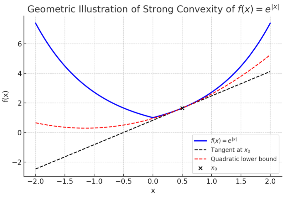
Strongly Convex Functions

Definition

A function $f: \text{dom}(f) \to \mathbb{R}$ is called strongly convex if there exists a parameter $\mu > 0$ such that for all $x, y \in \text{dom}(f)$ (where $\text{dom}(f)$ is a convex set):

$$f(y) \geq f(x) + \nabla f(x)^\top (y - x) + \frac{\mu}{2} \|y - x\|^2$$

Here, $\nabla f(x)$ is the gradient of $f$ at point $x$ (if $f$ is differentiable).

For non-differentiable functions, the subgradient version of the definition is: for all $g \in \partial f(x)$ (subdifferential), we have:

$$f(y) \geq f(x) + g^\top (y - x) + \frac{\mu}{2} \|y - x\|^2$$

💡 Intuitive explanation: A strongly convex function has a value at any point $x$ that is higher than a “strengthened” linear approximation (i.e., plus a quadratic term $\frac{\mu}{2} \|y - x\|^2$). This ensures the function has stronger curvature, leading to faster convergence in optimization.

Key Properties

(1) Strong Convexity Implies Strict Convexity

If $f$ is $\mu$-strongly convex, then it is also strictly convex. This means for all $x \neq y$ and $\lambda \in (0,1)$:

$$f(\lambda x + (1-\lambda) y) < \lambda f(x) + (1-\lambda) f(y)$$

Proof outline (from supplementary notes p15):
Assume $x \neq y$, let $z = \lambda x + (1-\lambda) y$. By strong convexity:

$$\begin{aligned} f(x) &> f(z) + \nabla f(z)^\top (x - z) \\ f(y) &> f(z) + \nabla f(z)^\top (y - z) \end{aligned}$$

Weighted average these two inequalities (weights $\lambda$ and $1-\lambda$), the gradient terms cancel, yielding:

$$\lambda f(x) + (1-\lambda) f(y) > f(z)$$

Thus proving strict convexity.

(2) Existence of a Unique Global Minimum

A strongly convex function has exactly one global minimum point $x^*$.
Proof outline (from supplementary notes p15):
Assume $x^*$ is a minimum point, then $\nabla f(x^*) = 0$ (differentiable case) or $0 \in \partial f(x^*)$ (non-differentiable case). By strong convexity:

$$f(y) \geq f(x^*) + \frac{\mu}{2} \|y - x^*\|^2$$

When $y \neq x^*$, $\frac{\mu}{2} \|y - x^*\|^2 > 0$, so $f(y) > f(x^*)$, meaning $x^*$ is unique.

Examples

A typical example of a strongly convex function is $f(x) = e^{|x|}$, which is strongly convex for some parameter $\mu$. Specifically, when $\mu = 1$, this function satisfies the strong convexity definition.

Applications in Optimization

Strong convexity significantly improves the convergence rate of optimization algorithms. Discussed in two cases:

(1) Gradient Descent for Smooth and Strongly Convex Functions

If $f$ is $L$-smooth and $\mu$-strongly convex (differentiable), then choosing step size $\eta = \frac{1}{L}$, the iterates of gradient descent satisfy:

$$\|x_{t+1} - x^*\|^2 \leq \left(1 - \frac{\mu}{L} \right) \|x_t - x^*\|^2$$

Error decays exponentially:

$$f(x_T) - f(x^*) \leq \frac{L}{2} \left(1 - \frac{\mu}{L} \right)^T \|x_0 - x^*\|^2$$

Proof:

From gradient descent update: $x_{t+1} = x_t - \eta \nabla f(x_t)$.
Consider distance change:

$$\|x_{t+1} - x^*\|^2 = \|x_t - \eta \nabla f(x_t) - x^*\|^2 = \|x_t - x^*\|^2 - 2\eta \nabla f(x_t)^\top (x_t - x^*) + \eta^2 \|\nabla f(x_t)\|^2$$

By strong convexity:

$$\nabla f(x_t)^\top (x_t - x^*) \geq f(x_t) - f(x^*) + \frac{\mu}{2} \|x_t - x^*\|^2$$

Substitute:

$$\|x_{t+1} - x^*\|^2 \leq \|x_t - x^*\|^2 - 2\eta \left( f(x_t) - f(x^*) + \frac{\mu}{2} \|x极 - x^*\|^2 \right) + \eta^极 \|\nabla f(x_t)\|^2$$

Rearrange:

$$\|x_{t+1} - x^*\|^2 \leq (1 - \mu \eta) \|x_t - x^*\|^2 - 2\eta (f(x_t) - f(x^*)) + \eta^2 \|\nabla f(x_t)\|^2$$

Now set $\eta = 1/L$. By smoothness, we have the sufficient decrease lemma:

$$f(x_{t+1}) \leq f(x_t) - \frac{1}{2L} \|\nabla f(x_t)\|^2$$

Thus, $-\frac{1}{2L} \|\nabla f(x_t)\|^2 \leq f(x_{极+1}) - f(x_t)$, but here we need to bound $\eta^2 \|\nabla f(x_t)\|^2$.

Actually, from smoothness:

$$f(x^*) \leq f(x_t) - \frac{1}{2L} \|\nabla f(x_t)\|^2$$

So $\|\nabla f(x_t)\|^2 \leq 2L (f(x_t) - f(x^*))$.

Substitute:

$$\eta^2 \|\nabla f(x_t)\|^2 = \frac{1}{L^2} \|\nabla f(x_t)\|^极 \leq \frac{2}{L} (f(x_t) - f(x^*))$$

Then:

$$\|x_{t+1} - x^*\|^2 \leq (1 - \mu \eta) \|x_t - x^*\|^2 - 2\eta (f(x_t) - f(x^*)) + \frac{2}{L} (f(x_t) - f(x^*))$$

Since $\eta = 1/L$, $-2\eta + \frac{2}{L} = 0$, so:

$$\|x_{t+1} - x^*\|^2 \leq (1 - \frac{\mu}{L}) \|x_t - x^*\|^2$$

This proves the first part.

For the second part, by smoothness:

$$f(x_T) -极 f(x^*) \leq \frac{L}{2} \|x_T - x^*\|^2 \leq \frac{L}{2} \left(1 - \frac{\mu}{L}\right)^T \|x_0 - x^*\|^2$$

Q.E.D.

Iteration requirement: To achieve error $\varepsilon$, the number of iterations needed is:

$$T \geq \frac{L}{\mu} \ln \left( \frac{R^2 L}{2\varepsilon} \right), \quad \text{where } R = \|x_0 - x^*\|$$

This is much faster than the non-strongly convex case (e.g., $\mathcal{O}(1/\varepsilon)$ rate for smooth convex functions), as the error decays as $\mathcal{O}(e^{-T})$.

(2) Subgradient Method for Strongly Convex Functions

If $f$ is $\mu$-strongly convex (possibly non-differentiable), and the subgradient norm is bounded (i.e., $\|g_t\| \leq B$ for all $g_t \in \partial f(x_t)$), then use decreasing step size:

$$\eta_t = \frac{2}{\mu(t + 1)}$$

And compute the weighted average point:

$$\bar{x}_T = \frac{2}{T(T+1)} \sum_{t=1}^T t \cdot x_t$$

The convergence rate is:

$$f(\bar{x}_T) - f(x^*) \leq \frac{2B^2}{\mu(T + 1)}$$

Proof:

From subgradient update: $x_{t+1} = x_t - \eta_t g_t$, where $g_t \in \partial f(x_t)$.
Consider distance change:

$$\|x_{t+1} - x^*\|^2 = \|x_t - \eta_t g_t - x^*\|^2 = \|x_t - x^*\|^2 - 2\eta_t g_t^\top (x_t - x^*) + \eta_t^2 \|g_t\|^2$$

By strong convexity:

$$g_t^\top (x_t - x^*) \geq f(x_t) - f(x^*) + \frac{\mu}{2} \|x_t - x^*\|^2$$

Substitute:

$$\|x_{t+极} - x^*\|^2 \leq \|x_t - x^*\|^2 - 2\eta_t \left( f(x_t) - f(x^*) + \frac{\mu}{2} \|x_t - x^*\|^2 \right) + \eta_t^2 \|g_t\|^2$$

Rearrange:

$$\|x_{t+1} - x^*\|^2 \leq (1 - \mu \eta_t) \|x_t - x^*\|^2 - 2\eta_t (f(x_t) - f(x^*)) + \eta_t^2 B^2$$

Now move terms:

$$2\eta_t (f(x_t) - f(x^*)) \leq (1 - \mu \eta_t) \|x_t - x^*\|^2 - \|x_{t+1} - x^*\|^2 + \eta_t^2 B^2$$

Substitute step size $\eta_t = \frac{2}{\mu(t+1)}$, then $1 - \mu \eta_t = 1 - \frac{2}{t+1} = \frac{t-1}{t+1}$.

Multiply both sides by $t$ (for telescoping):

$$2t \eta_t (f(x_t) - f(x^*)) \leq t(1 - \mu \eta_t) \|x_t - x^*\|^2 - t \|x_{t+1} - x^*\|^2 + t \eta_t^2 B^2$$

Note $t(1 - \mu \eta_t) = t \cdot \frac{t-1}{t+1} = \frac{t(t-1)}{t+1}$, and $t \eta_t^2 = t \cdot \frac{4}{\mu^2 (t+1)^2} = \frac{4t}{\mu^2 (t+1)^2}$.

But more directly, observe:

$$t(1 - \mu \eta_t) = \frac{t(t-1)}{t+1}, \quad \text{and} \quad (t+1) \|x_{t+1} - x^*\|^2 \text{ might appear}$$

Actually, from the original inequality:

$$2\eta_t (f(x_t) - f(x^*)) \leq \frac{\eta_t^2 B^2}{2} + \frac{1}{2\eta_t} \left( \|x_t - x^*\|^2 - \|x_{t+1} - x^*\|^2 \right) - \frac{\mu}{2} \|x_t - x^*\|^2$$

But the course material uses another approach.

According to the course material proof:
From the inequality:

$$f(x_t) - f(x^*) \leq \frac{B^2 \eta_t}{2} + \frac{\eta_t^{-1} - \mu}{2} \|x_t - x^*\|^2 - \frac{\eta_t^{-1}}{2} \|x_{t+1} - x^*\|^2$$

Substitute $\eta_t = \frac{2}{\mu(t+1)}$, then $\eta_t^{-1} = \frac{\mu(t+1)}{2}$.

So:

$$f(x_t) - f(x^*) \leq \frac{B^2}{2} \cdot \frac{2}{\mu(t+1)} + \frac{1}{2} \left( \frac{\mu(t+1)}{2} - \mu \right) \|x_t - x^*\|^2 - \frac{1}{2} \cdot \frac{\mu(t+1)}{2} \|x_{t+1} - x^*\|^2$$

Simplify:

$$f(x_t) - f(x^*) \leq \frac{B^2}{\mu(t+1)} + \frac{\mu}{4} \left( (t+1) - 2 \right) \|x_t - x^*\|^2 - \frac{\mu(t+1)}{4} \|x_{t+1} - x^*\|^2$$

i.e.:

f(x_t) - f(x^*) \leq \frac{B^2}{\极\mu(t+1)} + \frac{\mu}{4} (t-1) \|x_t - x^*\|^2 - \frac{\mu(t+1)}{4} \|x_{t+1} - x^*\|^2

Multiply both sides by $t$:

$$t (f(x_t) - f(x^*)) \leq \frac{t B^2}{\mu(t+1)} + \frac{\mu}{4} \left( t(t-1) \|x_t - x^*\|^2 - t(t+1) \|x_{t+1} - x^*\|^2 \right)$$

Sum from $t=1$ to $T$:

\sum_{t=1}^T t (f(x_t) - f(x^*)) \leq \sum_{t=1}^T \frac{t B^2}{\mu(t+1)} + \frac{\mu}{4} \left( \sum_{t=1}^T [t(t-1) \|x_t - x^*\|^2 - t(t+1) \极\|x_{t+1} - x^*\|^2] \right)

The second term on the right is a telescoping sum:

$$\sum_{t=1}^T [t(t-1) \|x_t - x^*\|^2 - t(t+1) \|x_{t+1} - x^*\|^2] = - T(T+1) \|x_{T+1} - x^*\|^2 \leq 0$$

Because when $t=1$, $1 \cdot 0 \cdot \|x_1 - x^*\|^2 = 0$, and subsequent terms cancel.

So:

$$\sum_{t=1}^T t (f(x_t) - f(x^*)) \leq \sum_{t=1}^T \frac{t B^2}{\mu(t+1)} \leq \frac{T B^2}{\mu}$$

By convexity, the weighted average satisfies:

$$f\left( \frac{2}{T(T+1)} \sum_{t=1}^T t x_t \right) \leq \frac{2}{T(T+1)} \sum_{t=1}^T t f(x_t)$$

So:

$$f\left( \frac{2}{T(T+1)} \sum_{t=1}^T t x_t \right) - f(x^*) \leq \frac{2}{T(T+1)} \sum_{t=1}^T t (f(x_t) - f(x^*)) \leq \frac{2}{T(T+1)} \cdot \frac{T B^2}{\mu} = \frac{2 B^2}{\mu (T+1)}$$

Q.E.D.

Iteration requirement: To achieve error $\varepsilon$, the number of iterations needed is $\mathcal{O}\left( \frac{B^2}{\mu \varepsilon} \right)$.

🔍 Note: Weighted averaging helps stabilize convergence and avoid subgradient oscillation. But the subgradient method is not a descent method, so averaging is necessary.

---

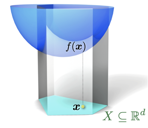
Projected Gradient Descent

Constrained Optimization Problem

$$\min_{x \in X} f(x)$$

where $X \subseteq \mathbb{R}^d$ is a closed convex set.

Projection Operator

The projection onto $X$ is defined as:

$$\Pi_X(y) = \arg\min_{x \in X} \|x - y\|$$

Update Rule

$$\begin{aligned} y_{t+1} &= x_t - \eta_t \nabla f(x_t) \\ x_{t+1} &= \Pi_X(y_{t+1}) \end{aligned}$$

Projection Properties

1. $(x - \Pi_X(y))^\top (y - \Pi_X(y)) \leq 0$ for all $x \in X$

2. $\|x - \Pi_X(y)\|^2 + \|y - \Pi_X(y)\|^2 \leq \|x - y\|^2$ for all $x \in X$

Proof:

1. Since $\Pi_X(y)$ minimizes $\|x - y\|^2$ over $X$, by optimality conditions, for any $x \in X$:

   $$(\Pi_X(y) - y)^\top (x - \Pi_X(y)) \geq 0$$

   i.e., $(x - \Pi_X(y))^\top (y - \Pi_X(y)) \leq 0$.

2. From 1, we have:

   $$\|x - y\|^2 = \|x - \Pi_X(y) + \Pi_X(y) - y\|^2 = \|x - \Pi_X(y)\|^2 + \|\Pi_X(y) - y\|^2 + 2 (x - \Pi_X(y))^\top (\Pi_X(y) - y)$$

   Since $(x - \Pi_X(y))^\top (\Pi_X(y) - y) \geq 0$, so:

   $$\|x - y\|^2 \geq \|x - \Pi_X(y)\|^2 + \|\Pi_X(y) - y\|^2$$

   i.e., property 2.

Convergence Rate

The convergence rate of projected gradient descent is the same as the unconstrained case, depending on function properties:

• If $f$ is convex and $L$-Lipschitz over $X$, error $O(1/\sqrt{T})$, iterations $O(1/\varepsilon^2)$.

• If $f$ is convex and $L$-smooth over $X$, error $O(1/T)$, iterations $O(1/\varepsilon)$.

• If $f$ is $\mu$-strongly convex and $L$-smooth over $X$, error $O(e^{-c T})$, iterations $O(\log(1/\varepsilon))$.

Proof sketch: Similar to unconstrained proof, but use projection properties to bound $\|x_{t+1} - x^*\|^2$. For example, for Lipschitz case:
From update:

$$y_{t+1} = x_t - \eta \nabla f(x_t)$$

By projection property 2:

$$\|x_{t+1} - x^*\|^2 \leq \|y_{t+1} - x^*\|^2 - \|y_{t+1} - x_{t+1}\|^2 \leq \|y_{t+1} - x^*\|^2$$

Then analyze similarly to unconstrained.

Summary Table

Function Properties	Algorithm	Convergence Rate	Iterations
Convex, $L$-Lipschitz	Gradient Descent	$f(x_{\text{best}}^{(T)}) - f(x^*) \leq \frac{RL}{\sqrt{T}}$	$O(1/\varepsilon^2)$
Convex, $L$-Smooth	Gradient Descent	$f(x_{\text{best}}^{(T)}) - f(x^*) \leq \frac{R^2 L}{2T}$	$O(1/\varepsilon)$
Convex, $L$-Lipschitz	Subgradient Method	$f(x_{\text{best}}^{(T)}) - f(x^*) \leq \frac{LR}{\sqrt{T}}$	$O(1/\varepsilon^2)$
$\mu$-Strongly Convex, $L$-Smooth	Gradient Descent	$f(x_{\text{best}}^{(T)}) - f(x^*) \leq \frac{RL}{2}(1 - \frac{\mu}{L})^T$	$O(\log(1/\varepsilon))$
$\mu$-Strongly Convex, $|g| \leq B$	Subgradient Method	$f(x_{\text{best}}^{(T)}) - f(x^*) \leq \frac{2B^2}{\mu(T+1)}$	$O(1/\varepsilon)$

Where $R = \|x_0 - x^*\|$.

Note: In practice, step size selection is crucial for convergence. For unknown parameters, adaptive step size strategies may be needed.

---

Additional Notes

1. Conflict between Strong Convexity and Lipschitz:
   Non-smooth functions cannot be both Lipschitz and strongly convex (e.g., $f(x) = \sqrt{x}$ is unbounded near $x=0$).

2. Relationship between Subgradient Norm and Lipschitz:

   • Lipschitz continuity $\Rightarrow$ bounded subgradient
   • Bounded subgradient $\not\Rightarrow$ Lipschitz continuity

3. Optimality:
   The convergence rates of first-order methods (gradient/subgradient) are optimal in general and cannot be further improved.

---