SDSC6015 Course 5-Mirror Descent and SDG

#sdsc6015

English / 中文

Mirror Descent

Click to expand Mirror Descent review content

Motivation

Consider the simplex-constrained optimization problem:

$$\min_{x \in \triangle_d} f(x)$$

where the simplex $\triangle_d := \{x \in \mathbb{R}^d : \sum_{i=1}^d x_i = 1, x_i \geq 0, \forall i\}$. Assume the gradient’s infinity norm is bounded: $\|\nabla f(x)\|_\infty = \max_{i=1,\ldots,d} |[\nabla f(x)]_i| \leq 1$.

• Notation: $x$ is the optimization variable, $d$ is the dimension, $\triangle_d$ is the probability simplex.

• Geometric Interpretation: The simplex is the space of probability distributions; constrained optimization aims to minimize the loss under probability constraints.

• Convergence Rate Comparison:

  • GD: $\mathcal{O}(\sqrt{d/T})$
  • Mirror Descent: $\mathcal{O}(\sqrt{\log d / T})$, superior in high-dimensional problems.

Preliminaries

• Dual Norm: $\|g\|_* = \sup_{\|x\| \leq 1} g^\top x$.

• Function Properties:

  • $L$-Lipschitz: $\|g\|_* \leq L$ for $g \in \partial f(x)$.
  • $\beta$-smooth: Gradient satisfies Lipschitz condition.
  • $\mu$-strongly convex: Function has a lower-bounding quadratic term.

Mirror Descent Algorithm

Iteration format:

$$y_{t+1} = \nabla \Phi^*( \nabla \Phi(x_t) - \eta g_t ), \quad x_{t+1} = \Pi_X^\Phi(y_{t+1})$$

where $g_t \in \partial f(x_t)$, $\Phi$ is the mirror potential, $\Pi_X^\Phi$ is the projection based on Bregman divergence.

• Notation: $\Phi$ is strictly convex and continuously differentiable, $D_\Phi(x,y)$ is the Bregman divergence.

• Geometric Interpretation: Transforms the problem into the dual space via the potential function, making the update direction better align with the geometric structure.

Convergence Theorem

Theorem 1 (Mirror Descent Convergence):
Let $\Phi$ be a $\rho$-strongly convex mirror map, $R^2 = \sup_{x \in X} \Phi(x) - \Phi(x_1)$, $f$ convex and $L$-Lipschitz. Choose $\eta = \frac{2R}{L} \sqrt{\frac{\rho}{T}}$, then:

$$\min_{t=1,\ldots,T} \mathbb{E}[f(x_t)] - f(x^*) \leq 2RL \sqrt{\frac{1}{\rho T}}$$

Proof Outline

1. Utilize the strong convexity of the Bregman divergence to bound the error. 2. Control terms via gradient Lipschitz properties. 3. Summation and step size optimization. For details, see Document 1, Page 9.

Standard Settings

• Ball Setting: $\Phi(x) = \frac{1}{2} \|x\|_2^2$, equivalent to projected gradient descent.

• Simplex Setting: $\Phi(x) = \sum_{i=1}^d x_i \log x_i$ (negative entropy), Bregman divergence is KL divergence, projection achieved via renormalization.

• Example: When optimizing probability distributions on the simplex, Mirror Descent naturally handles constraints, preventing Euclidean projection bias.

---

Stochastic Gradient Descent (SGD)

---

Problem Formulation

The main problem is defined as minimizing a function $f(\theta)$, where $\theta \in \mathbb{R}^d$ is the parameter vector. The specific form is:

$$\underset{\theta \in \mathbb{R}^d}{\text{minimize}} \, f(\theta)$$

Here, $f(\theta)$ is typically an expected loss function, expressed as:

$$f(\theta) = \int \ell(\theta, Z) \, dP(Z)$$

• $Z \in \mathbb{R}^p$ is a random variable representing a data point (e.g., features and labels).

• $P(Z)$ is the unknown distribution, reflecting that in real-world problems the data distribution is often unknown and must be estimated from samples.

• $\ell(\theta, Z)$ is the loss function, parameterized by $\theta$, used to measure the model’s performance on data point $Z$.

Core Idea: Learn parameters $\theta$ by minimizing the expected loss, but since $P(Z)$ is unknown, empirical risk minimization is used in practice, approximating the integral with the sample mean.

Given a set of labeled training data $(x_1, y_1), \ldots, (x_n, y_n) \in \mathbb{R}^d \times \mathcal{Y}$, the goal is to find the weight parameters $\theta$ to classify the data. This connects the optimization problem with supervised learning tasks like classification or regression.

In simple terms, the main problem is to optimize parameters $\theta$ to minimize the model’s average loss over all possible data, but due to the unknown distribution, we rely on finite samples.

---

Motivation

When the dataset is huge (e.g., $n \gg 1,000,000$), computing the full gradient becomes impractical. Specific analysis:

• Define $f_i(\theta) = \ell(\theta, (x_i, y_i))$ as the cost function for the $i$-th observation, drawn from a training set of $n$ observations.

• The full gradient $\nabla f(\theta) = \sum_{i=1}^n \nabla f_i(\theta)$ requires iterating over all data points; the computational cost grows linearly with $n$, creating a bottleneck when $n$ is very large.

• Therefore, cheaper methods can be used: compute the gradient of a single component $\nabla f_i(\theta)$ or a mini-batch gradient. This introduces Stochastic Gradient Descent (SGD) or its variants, which approximate the gradient by randomly sampling a subset of data points, significantly reducing the computational cost per iteration.

---

SGD Algorithm Description

The basic steps of stochastic gradient descent are as follows:

• Initialization: Set the initial point $x_0 \in \mathbb{R}^d$.

• Iteration Process: For each time step $t = 0, 1, \ldots$:

  • Randomly and uniformly sample an index $i_t \in \{1, 2, \ldots, n\}$.
  • Update parameters: $x_{t+1} = x_t - \eta_t \nabla f_{i_t}(x_t)$, where $\eta_t$ is the learning rate.

Here, $g_t := \nabla f_{i_t}(x_t)$ is called the stochastic gradient; it uses the gradient of only a single function component $f_{i_t}$, not the full gradient $\nabla f(x_t) = \frac{1}{n} \sum_{i=1}^n \nabla f_i(x_t)$.

Advantage: Computational Efficiency

• Each iteration computes the gradient of only one function component, so the iteration cost is $n$ times lower than Full Gradient Descent.
• This makes SGD more scalable for large datasets.

Convergence Considerations

Although SGD is computationally efficient, using the gradient of a single component does not guarantee convergence. The document provides an example to illustrate this issue:

Example: Consider the optimization problem $\min_x f(x) = f_1(x) + f_2(x)$, where $f_1(x) = x^2$ and $f_2(x) = -x^2$. If starting from $x_k > 0$ and randomly sampling $i_k = 2$, the gradient update $x_{k+1} = x_k - \eta_t \nabla f_2(x_k)$ may cause the function value to increase (because $\nabla f_2(x) = -2x$, the update direction might be wrong).

However, SGD can produce descent in expectation, leading to the concept of unbiasedness.

Unbiasedness

The stochastic gradient $g_t$ is an unbiased estimator of the true gradient $\nabla f(x_t)$, i.e.:

$$\mathbb{E}[g_t|x_t = x] = \nabla f(x_t)$$

where the expectation is taken over the random index $i_t$.

Significance: Unbiasedness ensures that on average, the update direction of SGD is correct. Although individual steps may randomly deviate, in the long run, the algorithm converges towards the optimal solution. This allows the use of expectation inequalities to analyze convergence, rather than relying on strong assumptions like convexity.

---

Conditional Expectation

Detailed Explanation of Conditional Expectation:

Definition

Conditional expectation is a core concept in probability theory and statistics, used to approximate a random variable given partial information (e.g., the value of another random variable).

• Definition: Let X and Y be random variables. The conditional expectation of X given Y, denoted $E[X|Y]$, is the best approximation of X using only the information from Y.

  • This differs from the unconditional expectation $E[X]$: $E[X]$ gives the overall average of X, while $E[X|Y]$ gives the average of X given the value of Y.
  • Intuitively, conditional expectation “filters out” the influence of Y, providing a more precise local estimate.

Explanation: Conditional expectation is commonly used in machine learning to handle partially observed data, such as optimizing model parameters in stochastic gradient descent.

Properties

• Linearity: Conditional expectation is linear, i.e., for random variables X and Y, and constants a and b:

  $$E[aX + bY | Z] = aE[X|Z] + bE[Y|Z]$$

  The document implies similar properties, e.g., for Z = X + Y or Z = XY, conditional expectation may satisfy addition or multiplication rules, but specific formulas are not given.

• Partition Theorem: For discrete random variable Y, this theorem provides a simplified method for computing expectations.

  • Theorem statement: If Y is a discrete random variable, then the unconditional expectation can be computed via the expectation of the conditional expectation, i.e.:

    $$E[X] = E[E[X|Y]]$$

    This means first compute the conditional expectation of X given Y, then take the expectation over Y.
  • A footnote in the document indicates that formal definitions and properties can be found in relevant textbooks; this theorem is a special case of the Law of Total Expectation.

Example: Suppose Y is discrete (e.g., a categorical variable), then $E[X]$ can be obtained by computing $E[X|Y=y]$ for each possible value of Y and taking a weighted average.

Convexity of Expectation

• For any fixed x, the linearity of conditional expectation allows simplification of calculations:

$$E[f(X)|Y] = \text{linear combination based on Y}$$

where f is a convex function.

• The document mentions that the event $\{x_t = x\}$ occurs only for x in a finite set X (i.e., $x_t$ is determined by the index selections from previous iterations). This implies that in iterative algorithms (like stochastic gradient descent), parameter updates are limited to a finite number of options.

• Application of the Partition Theorem: By decomposing the expectation into conditional expectations, convexity analysis can be simplified. For example:

$$E[L(x_t)] = E[E[L(x_t)|Y]]$$

where L is the loss function, aiding in convergence proofs.

Explanation: In stochastic optimization, this convexity analysis ensures algorithm stability and convergence even with noisy data.

Summary

The document focuses on the definition and properties of conditional expectation (such as linearity and the Partition Theorem) and its application in convexity analysis. These concepts are fundamental to stochastic optimization and machine learning, helping to handle uncertainty and partial information. Conditional expectation, as a “best approximation” tool, plays a key role in model training and convergence proofs.

Note: Image labels mentioned in the document (such as ``) are not embedded in the summary as the specific content is not provided, and to avoid fabrication. The summary is strictly based on the text content.

---

Convergence Theorems

Theorem 2 (SGD on Convex Functions):
Let $f$ be convex and differentiable, $x^*$ be the global optimum, $\|x_0 - x^*\| \leq R$, and $\mathbb{E}[\|g_t\|^2] \leq B^2$. Choose constant step size $\eta = \frac{R}{B \sqrt{T}}$, then:

$$\frac{1}{T} \sum_{t=0}^{T-1}\mathbb{E} \left[ f(x_t) \right] - f(x^*) \leq \frac{RB}{\sqrt{T}}$$

Proof Details (Supplemented from Document2 P23)

Proof Outline:

1. Basic Inequality: Start from the iteration rule:

   $$\|x_{t+1} - x^*\|^2 = \|x_t - x^*\|^2 - 2\eta g_t^\top (x_t - x^*) + \eta^2 \|g_t\|^2$$

2. Take Expectation: Utilize unbiasedness $\mathbb{E}[g_t | x_t] = \nabla f(x_t)$ and convexity expectation:

   $$\mathbb{E}[g_t^\top (x_t - x^*)] = \mathbb{E}[\nabla f(x_t)^\top (x_t - x^*)] \geq \mathbb{E}[f(x_t) - f(x^*)]$$

3. Summation and Optimization: Sum from $t=0$ to $T-1$, and substitute step size $\eta = \frac{R}{B \sqrt{T}}$:

   $$\sum_{t=0}^{T-1} \mathbb{E}[f(x_t) - f(x^*)] \leq \frac{R^2}{2\eta} + \frac{\eta B^2 T}{2} = RB \sqrt{T}$$

4. Jensen’s Inequality: Apply $\mathbb{E}[f(\bar{x}_T)] \leq \frac{1}{T} \sum_{t=0}^{T-1} \mathbb{E}[f(x_t)]$ to obtain the final bound.

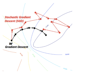
Geometric Interpretation: SGD moves in a descent direction in expectation, but variance causes oscillations; the step size balances convergence speed and stability.

• Notation: $R$ is the initial error bound, $B$ is the stochastic gradient norm bound, $T$ is the number of iterations.

• Comparison with GD: The full gradient descent norm bound $B_{\text{GD}}^2$ is usually smaller than SGD’s $B_{\text{SGD}}^2$ (due to Jensen’s inequality), but SGD has lower cost per round, resulting in higher overall efficiency.

Theorem 3 (SGD on Strongly Convex Functions):
Let $f$ be $\mu$-strongly convex, $x^*$ be the unique optimum, choose step size $\eta_t = \frac{1}{\mu t}$, then:

$$\mathbb{E}[\|x_T - x^*\|^2] \leq \frac{B^2}{\mu^2 T}$$

Proof Details (Supplemented from Document2 P26)

Proof Steps:

1. Strong Convexity Inequality:

   $$f(x^*) \geq f(x_t) + \nabla f(x_t)^\top (x^* - x_t) + \frac{\mu}{2} \|x_t - x^*\|^2$$

2. Iteration Analysis: Substitute the SGD update rule, take expectation:

   $$\mathbb{E}[\|x_{t+1} - x^*\|^2] \leq (1 - \mu \eta_t) \mathbb{E}[\|x_t - x^*\|^2] + \eta_t^2 B^2$$

3. Recursive Solution: Set $\eta_t = 1/(\mu t)$, use the recurrence relation and summation to obtain the convergence bound.

Geometric Interpretation: Strong convexity ensures the function has a unique minimum; SGD converges at a linear rate, but the variance term $B^2$ affects precision.

Mini-batch SGD

Use batch update: $\tilde{g}_t = \frac{1}{|S_t|} \sum_{i \in S_t} \nabla f_i(x_t)$, where $S_t \subset \{1, \ldots, n\}$ is a random subset.

• Notation: $|S_t| = m$ is the batch size, $m=1$ is equivalent to SGD, $m=n$ is equivalent to GD.

• Variance Calculation (Supplemented from Document2 P31):

  $$\mathbb{E}[\|\tilde{g}_t - \nabla f(x_t)\|^2] = \frac{1}{m} \mathbb{E}[\|\nabla f_1(x_t) - \nabla f(x_t)\|^2] \leq \frac{B^2}{m}$$

  As $m \to \infty$, the variance tends to zero.

• Geometric Interpretation: Batch averaging reduces variance, making the gradient estimate more stable, but increases computational cost per round.

Stochastic Subgradient Descent and Constrained Optimization

For non-smooth problems, use subgradient $g_t \in \partial f_i(x_t)$, update: $x_{t+1} = x_t - \eta_t g_t$. For constrained problems, add a projection step (Projected SGD), convergence rate remains $\mathcal{O}(1/\varepsilon^2)$.

---

Momentum Methods

Motivation

GD oscillates severely on long, narrow valley-shaped functions. Momentum methods introduce historical step information to accelerate convergence.

• Geometric Interpretation: Momentum acts like an inertial ball, accelerating in flat directions and damping in steep directions, reducing oscillations.

Heavy Ball Method (Polyak Momentum)

Update rule:

$$x_{t+1} = x_t - \eta_t \nabla f(x_t) + \beta_t (x_t - x_{t-1})$$

Or equivalently:

$$v_{t+1} = \beta_t v_t - \eta_t \nabla f(x_t), \quad x_{t+1} = x_t + v_{t+1}$$

where $\beta_t \in [0,1]$ is the momentum coefficient.

• Notation: $v_t$ is the momentum term, $\beta_t$ controls the weight of history.

• Geometric Interpretation: The momentum term retains the previous direction, helping to traverse locally flat regions.

Convergence

Theorem 4 (Convergence on Quadratic Functions):
Consider the strongly convex quadratic function $f(x) = \frac{1}{2} x^\top Q x - b^\top x$, where $Q$ is positive definite, condition number $\kappa = L/\mu$. Choose $\eta_t = \frac{4}{(\sqrt{L} + \sqrt{\mu})^2}$, $\beta_t = \left( \frac{\sqrt{\kappa} - 1}{\sqrt{\kappa} + 1} \right)^2$, then the heavy ball method converges at a linear rate.

Proof Outline

Proof Idea:

• Through eigenvalue analysis, the momentum term improves the convergence constant of GD.

• Detailed proof can be found in Document 1, Page 39, and references (e.g., Wright & Recht, 2022).

Geometric Interpretation: For quadratic functions, momentum adjusts the step size to match the eigenvalue distribution of the Hessian matrix, accelerating convergence.

• Counterexample (Document 1, Pages 41-44): For a piecewise quadratic function $f(x)$, although it is 1-strongly convex and 25-smooth, the heavy ball method may cycle without converging (e.g., with $\eta_t = 1/9$, $\beta_t = 4/9$, $x_0 = 3.3$, iterations may cycle among three points).

  • Geometric Interpretation: Non-smooth points cause incorrect momentum directions, leading to oscillations.
  • Schematic Diagram:
    ![Potential oscillation diagram description - specific image content not provided]

Nesterov’s Accelerated Gradient Descent

Similar to the heavy ball method but uses a lookahead point to compute the gradient, with more robust theoretical guarantees. Update rule difference:

• Heavy Ball: Directly combines current gradient and momentum.

• Nesterov’s Method: First moves along the momentum direction, then computes a gradient correction.

• Geometric Interpretation: Nesterov’s method reduces oscillation through “lookahead” steps, making it more suitable for general convex functions.

---